Tutorial: Parallelization concepts🔗
Early Adopter restriction
The examples below still refer to HDevelop and its language, not HDevelopEVO and HALCON Script.
The general concepts, however, are valid for both HDevelop and HDevelopEVO.
Parallelization can be performed by several means, depending on the specific application and the goal of the parallelization.
Only a selection of the most common general concepts can be provided.
The parallelization concepts relate to the specific goals of the parallelization:
However, in practice you will often want to find a compromise between different goals.
Minimizing the response time🔗
Basic concepts to minimize the response time of an application are data parallelization and task parallelization.
Data parallelization and automatic operator parallelization🔗
Data parallelization means that multiple threads perform the same task on different pieces of data.
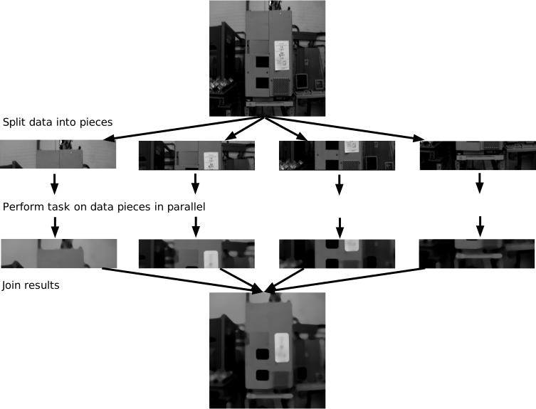
Figure 1 shows the concept of data parallelization: First, the data is split into several data pieces of approximately the same size. Then, the task is performed for each data piece individually by different threads. Finally, after the last thread has finished, the results of all threads are joined.
By default, almost all operators automatically perform a data parallelization.
Tip
In many cases, HALCON’s automatic operator parallelization (AOP) is efficient enough so that a manual implementation of data parallelization does not lead to any further runtime enhancement.
For more information on this topic, see automatic parallelization.
The following example explains the concept by manually implementing data parallelization for a median filter.
Simulating AOP
The HDevelop example program hdevelop/System/Parallelization/simulate_aop.hdev shows how to implement data parallelization for a median filter (see also Figure 1) and compares the runtime with the runtime needed for the sequential processing and for HALCON’s AOP.
To use AOP, the system parameter 'parallelize_operators' must be set to 'true', which is the default.
The number of threads to be used can be set explicitely by setting the system parameter 'thread_num' to a value between 1 and the available number of cores.
By default, all available cores are used for AOP.
set_system ('parallelize_operators', 'true')
median_image (Image, ImageMedianAop, 'circle', Radius, 'mirrored')
The following code shows an implementation of data parallelization by simulating AOP.
To achieve this, AOP is turned off first.
Then, the image is split into pieces of approximately the same size.
This is done by reducing the domains of the images to be handled by the individual threads to a respective sub-region of the domain of the input image.
With the qualifier par_start , the individual threads that run in parallel are started.
In each thread, the median is calculated for the corresponding part of the image.
The results of the different threads are collected using vector variables.
get_system ('processor_num', Cores)
MaxNumberOfSubthreads := 20
MaxThreads := min([Cores,MaxNumberOfSubthreads])
set_system ('parallelize_operators', 'false')
for Threads := 1 to MaxThreads by 1
        get_region_runs (Image, Row, ColumnBegin, ColumnEnd)
        RunsPerThread := |Row| / Threads
        * Split up the image and process each region by a separate thread:
        for Thread := 0 to Threads - 1 by 1
            IndexStart := Thread * RunsPerThread
            if (Thread < Threads - 1)
                IndexEnd := IndexStart + RunsPerThread - 1
            else
                IndexEnd := |Row| - 1
            endif
            gen_region_runs (Region, Row[IndexStart:IndexEnd], \
                             ColumnBegin[IndexStart:IndexEnd], \
                             ColumnEnd[IndexStart:IndexEnd])
            reduce_domain (Image, Region, ImageReduced)
            par_start<ThreadID.at(Thread)> : median_image (ImageReduced, \
                                  ImageMedianThread.at(Thread), 'circle', \
                                  Radius, 'mirrored')
        endfor
        convert_vector_to_tuple (ThreadID, ThreadIDs)
endfor
To wait until all involved threads are finished, the operator par_join is called.
Then, the results of the individual threads are copied into one image.
par_join (ThreadIDs)
* Free references to thread IDs.
ThreadID.clear()
ThreadIDs := []
* Merge results
full_domain (ImageMedianThread.at(0), ImageMedianPar)
for ImagePart := 1 to Threads - 1 by 1
    overpaint_gray (ImageMedianPar, ImageMedianThread.at(ImagePart))
endfor
The runtimes of the different cases are visualized in Figure 2 for a machine with four cores.
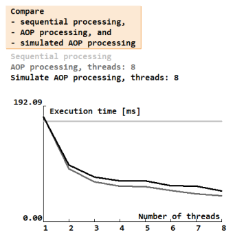
The manual parallelization has no advantage compared to the automatic operator parallelization. Due to some overhead caused by HDevelop, the runtime of the simulated AOP processing is even slightly larger than that of the AOP. However, both are significantly faster than the sequential processing.
Task parallelization🔗
Task parallelization means that different tasks are performed in different threads, for example, on the same image (see Figure 3).
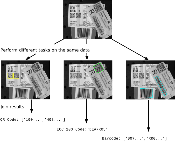
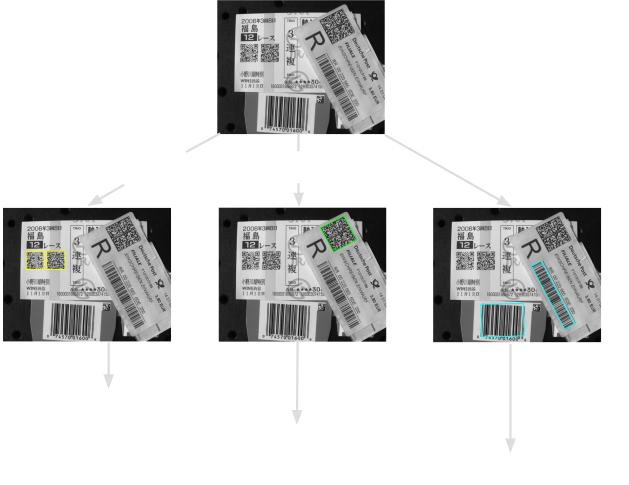
The following example shows the usage of par_start and par_join to parallelize tasks.
Task parallelization
The HDevelop example program hdevelop/Control/par_start.hdev reads bar codes and different types of 2d codes in parallel.
After the creation and training of the bar code and 2d code models, for each reading task a corresponding procedure is called in a separate thread using the par_start qualifier: a procedure to read bar codes, a procedure to read Data Matrix codes, and a procedure to read QR codes.
The operator par_join waits for all sub-threads to finish before the results of the individual threads are used for further processing (for example, displaying the results).
par_start<ThreadQRCode> : find_qr_codes (Image, QrCodeXlds, QrCodeModel, \
                                         QrCodeHandlesSeq, \
                                         QrCodeStringsSeq)
par_start<ThreadECC200> : find_ecc200_codes (Image, Ecc200Xlds, Ecc200Model, \
                                             Ecc200Handles, Ecc200Strings)
par_start<ThreadBarcode> : find_bar_codes (Image, BarCodeRegions, \
                                           BarCodeModel, BarCodeStrings)
par_join ([ThreadQRCode,ThreadECC200,ThreadBarcode])
dev_display (QrCodeXlds)
dev_display (Ecc200Xlds)
dev_display (BarCodeRegions)
The example program not only shows how to parallelize the three identification tasks, but also provides hints for which kinds of tasks parallelization is reasonable. Additionally, the speedup of the parallelization is demonstrated by a comparison of the runtimes needed for the parallelized procedure calls and the corresponding sequentially applied procedure calls.
Maximizing throughput via pipelining🔗
When dealing with streaming data, the throughput of a system is often more important than its response time. One way to increase the throughput of a system is pipelining.
Pipelining is frequently associated with the processing of streaming data, like images taken from a camera that monitors objects on a conveyor belt (compare Figure 4).
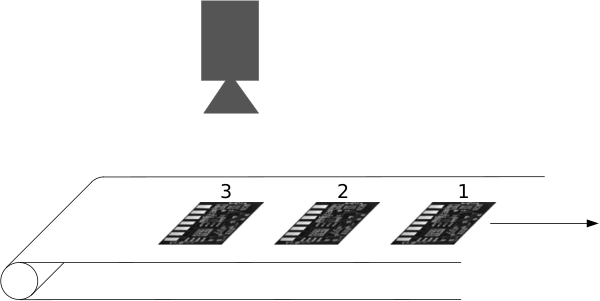
In this case, the image of object 3 may be acquired at the same time as the image of object 2 is processed, and at the same time as the image processing results of object 1 are evaluated.
Basic design of a pipeline🔗
The individual processing steps, for example, image acquisition, image processing, and result evaluation, are executed by different stages that are connected by message queues. The output of one stage then becomes the input of the next one. Thus, a pipeline is composed of (typically) multiple producer/consumer pairs.
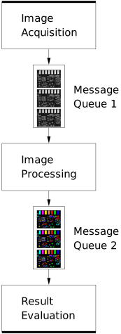
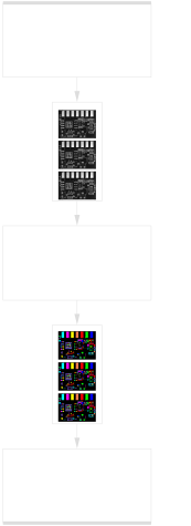
The pipeline in Figure 5 consists of three stages, which are connected by two message queues.
All three stages run in separate threads that run in parallel.
The image acquisition stage acquires the images.
Each image is put into a message, which then is enqueued into the message queue 1.
The message queues act as FIFO (first in, first out) buffers, which connect the consecutive stages.
If the image processing stage is ready to process the next image and as soon as there is a message available in message queue 1, the image processing stage dequeues a message from the head of message queue 1.
It processes the image that is contained in the message and adds the processing results to the message.
Then it enqueues this message to message queue 2.
Finally, the result evaluation stage dequeues the message from the head of message queue 2 and evaluates the results, for example, by initiating some action like blowing-out defective products.
As the threads run in parallel, the result evaluation for the first image may be executed parallel to the processing of the second image and parallel to the acquisition of the third image. Typically, the processing time of the different stages is unequal. For example, in Figure 6, the image processing stage takes twice as long as the result evaluation stage.
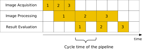
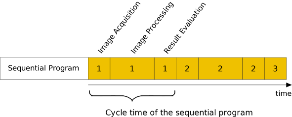
As the individual stages of a pipeline are executed in parallel, its throughput is typically higher than the throughput of a program that executes the stages sequentially (see Figure 7).
Example implementation of the pipeline🔗
The implementation of a pipeline follows this pattern:
- Put the functionality of the stages into individual procedures.
- Create and configure message queues.
- Prepare data structures for a clean termination of the pipeline.
- Start the procedures in individual threads.
The following example explains the HDevelop example program hdevelop/System/Multithreading/pipeline_one_thread_per_stage.hdev, which shows an implementation of a pipeline similar to the one referred to in Figure 5 and Figure 6.
Simple pipeline
First, the functionality of the different stages has to be put into individual procedures.
Here, the three procedures acquire_images, process_images, and evaluate_results are used.
The data that must be passed from one stage to the next stage will be passed through message queues.
As we have three stages, we need two message queues to connect theses stages.
They are created with the operator create_message_queue:
create_message_queue (QueueOriginalImage)
create_message_queue (QueueImageProcessingResult)
Typically, the size of the message queues should be limited to control the memory usage of the program. This is done by the following calls:
MessageQueueMaxMessageNum := 200
set_message_queue_param (QueueOriginalImage, 'max_message_num', \
                         MessageQueueMaxMessageNum)
set_message_queue_param (QueueImageProcessingResult, 'max_message_num', \
                         MessageQueueMaxMessageNum)
Choose the size of the message queues large enough to allow them to handle short-term peak loads. If, for example, the images are acquired faster than they can be processed for a short period of time, they will be buffered in the message queue.
To be able to stop the image acquisition, we use an event that is monitored inside the procedure acquire_images:
create_event ('', '', StopAcq)Furthermore, we propagate the information that the image acquisition has been stopped with a respective message.
This message is created by the image acquisition stage as soon as the image acquisition is stopped.
It indicates that no further messages will follow. To identify this message, we define a particular message key:
TerminationKey := 'terminate'Then, we can start the procedures in individual threads:
par_start<AcquisitionThread> : acquire_images (MeanAcquisitionInterval, \
                                               StopAcq, TerminationKey, \
                                               QueueOriginalImage)
par_start<ImageProcessingThread> : process_images (QueueOriginalImage, \
                                                   NumAOPThreadsForImageProcessing, \
                                                   TerminationKey, \
                                                   QueueImageProcessingResult)
par_start<ResultEvaluationThread> : evaluate_results (QueueImageProcessingResult, \
                                                      TerminationKey, \
                                                      WindowHandle)
In the example program, the pipeline runs just a few seconds and is then terminated by signaling the event StopAcq:
signal_event (StopAcq)Now, the image acquisition stage, which monitors the state of the event StopAcq, terminates and sends a message to the subsequent stages, which will terminate themselves as soon as they evaluate this message.
Finally, we must wait until all threads are finished.
par_join ([AcquisitionThread,ImageProcessingThread,ResultEvaluationThread])Example implementation of the image acquisition stage🔗
The implementation of the first stage (here represented by the procedure acquire_images) follows this pattern:
- Acquire data.
- Create new message.
- Add data and meta information to the message.
- Enqueue the message to the output message queue.
- Check and handle the event that signals the termination of the stage.
In the following example, the image acquisition stage acquires images in a loop. The loop is not exited until either
- the image acquisition is terminated by signaling the termination event or
- the message queue that connects the image acquisition stage with the image processing stage reaches its limit.
Image acquisition stage
In our example, the image acquisition is simulated by picking a random image from an array of pre-read images and waiting some time to simulate a realistic time interval between the acquisition of two images. In real applications, these two lines must be replaced to acquire real images.
repeat
    wait_to_simulate_non_trivial_acquisition_time (MeanAcquisitionInterval, \
                                                   ImageId, \
                                                   LastAcquisitionTime, \
                                                   LastAcquisitionTime)
    acquire_random_image (Images, Image)
For each image, we create a message and store the image together with an image ID and a time stamp in this message:
    create_message (MessageImg)
    set_message_obj (Image, MessageImg, 'image')
    set_message_tuple (MessageImg, 'image_id', ImageId)
    set_message_tuple (MessageImg, 'acquisition_time', AcquisitionTime)
Finally, the message is enqueued into the message queue that connects the image acquisition stage with the image processing stage. Because the size of our message queues is limited, we must take care of the case that the message queue already contains its maximally allowed number of messages. For this, we use a procedure that can be configured to handle this case in the desired way:
    enqueue_message_to_limited_queue (MessageImg, QueueOut, \
                                      'throw_exception')
Note
Here, we want to throw an exception if the message queue is at its limit. In real applications, this case must be handled individually and with care. It indicates that one of the following stages cannot handle the images in the required speed. Because the reduction of the image acquisition rate is most often not the desired solution, the speed of the pipeline must be increased. See Speeding up the pipeline for possible options.
Finally, we check if the image acquisition should be terminated by checking the state of the event StopAcq.
As long as this event is not signaled, the image acquisition stage continues to acquire images:
    try_wait_event (StopAcq, Busy)
until (not Busy)
If the event StopAcq is signaled, the image acquisition loop will be left and the complete pipeline can be terminated.
To do this in a way that all acquired images are still being processed, we create a message that contains the above defined termination key and enqueue it as the final message to the message queue.
In this case, we must ensure that the message will be enqueued to the message queue.
Therefore, we do not want to throw an exception if the message queue is at its limit but rather wait until the message can be enqueued:
create_message (TerminationMessage)
set_message_tuple (TerminationMessage, TerminationKey, 'true')
enqueue_message_to_limited_queue (TerminationMessage, QueueOut, 'wait')
Example implementation of the image processing stage🔗
The implementation of intermediate stages (here represented by the procedure process_images) follows this pattern:
- Dequeue a message from the input message queue.
- Process the data contained in the message.
- Add processing results to the message.
- Enqueue the message to the output message queue.
In the following example, all these steps are performed inside a loop, which exits if the pipeline is terminated.
Image processing stage
First, a message is dequeued from the input message queue:
while (1)
    dequeue_message (QueueIn, [], [], MessageHandle)
Then, we check if the image acquisition was terminated and thus we have to terminate the pipeline:
    get_message_param (MessageHandle, 'key_exists', TerminationKey, \
                       Terminate)
If we have to terminate the pipeline, the following steps are needed:
- Enqueue the termination message to the output queue to inform subsequent stages about the termination.
- Exit the loop.
    if (Terminate)
        enqueue_message_to_limited_queue (MessageHandle, QueueOut, 'wait')
        break
    endif
If no termination was requested, we can extract the input data (here: image) from the message, perform some action (here: image processing), and add the result (here: number of defects) to the message:
    get_message_obj (Image, MessageHandle, 'image')
    image_processing (Image, ImageReduced, RegionUnion, RingSize, \
                      PolarResolution, SmoothX, Number)
    set_message_tuple (MessageHandle, 'num_defects', Number)
Finally, we enqueue the message to the output queue:
    enqueue_message_to_limited_queue (MessageHandle, QueueOut, 'wait')
endwhile
Here, it is not necessary to throw an exception if the output queue reached its limit. We just wait until we can enqueue the message. As long as we are waiting, we cannot dequeue further messages from the input queue. If this waiting state takes too long, the input queue will reach its limit and a respective exception will be thrown by the image acquisition stage.
Example implementation of the result evaluation stage🔗
The implementation of the final stage (here represented by the procedure evaluate_results) follows this pattern:
- Dequeue a message from the input message queue.
- Process the data contained in the message.
In the following example, all these steps are performed inside a loop, which is not exited until the pipeline is terminated.
Image evaluation stage
First, a message is dequeued from the input message queue:
while (1)
    dequeue_message (QueueIn, [], [], MessageHandle)
Then we check if the image acquisition was terminated and thus we have to terminate the pipeline:
    get_message_param (MessageHandle, 'key_exists', TerminationKey, \
                       Terminate)
    if (Terminate)
        break
    endif
endwhile
Now, we can evaluate the results. In the example, we just calculate response time, processing time, and the mean acquisition interval and visualize the data. In real applications, the results can be used to control the elimination of defective parts, for example.
Runtime behavior🔗
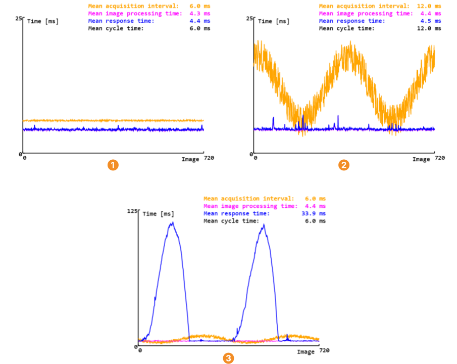
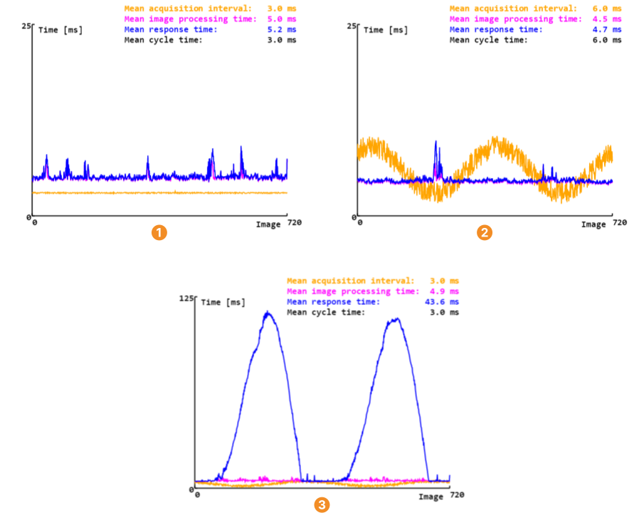
Figure 8 shows the runtime behavior of the simple pipeline realized in the example program described above.
On the horizontal axis, the last 720 images are plotted.
The orange line shows the acquisition interval, that is, the time between the acquisition of two consecutive images.
The acquisition interval shows some variations, which are specifically caused by the image acquisition procedure.
The magenta line shows the time needed for the image processing stage, which is fairly constant over the images.
The blue line shows the response time, that is, the time between the image acquisition and the completion of the result evaluation.
Approximately constant acquisition interval
The images are acquired in approximately equal intervals of 6 ms.
Note that the image acquisition must not be faster than the slowest of the following stages of the pipeline.
In our example, this stage is the image processing stage, which takes about 4.5 ms.
With the above mentioned image acquisition interval of 6 ms, we can achieve a throughput of \(\frac{1}{6\,{\rm ms}} \approx 160 \,\) images\(/\rm s\) with a nearly constant response time.
Varying acquisition interval
As long as the pipeline (more precisely: the slowest stage following the image acquisition stage) is fast enough, this has no negative effect on the response time.
This can be seen in figure
, where the images are always acquired slower than they are processed.
This limits the achievable throughput, because at any time, the image acquisition speed may not exceed the speed of the following stages.
In this configuration of our example, only \(\frac{1}{12\,{\rm ms}} \approx 80 \,\) images\(/\rm s\) can be processed, again with a nearly constant response time.
Varying acquisition interval leading to short-term peak loads
If the response time is less important, the image acquisition interval can even drop below the time required to process one image for a limited period of time.
As long as the image processing is faster than the image acquisition (magenta line is below the orange line), the response time is only marginally above the image processing time.
In this case, the message queues contain typically at most one message.
As soon as the acquisition interval is shorter than the time required to process one image, the acquired images must be buffered in the input message queue of the image processing stage.
The response time for those images, which must wait in the message queue for being processed, increases dramatically.
As soon as the image acquisition is again slower than the image processing, the number of buffered images decreases and with this also the response time for newly acquired images.
Note that the message queues must be configured large enough to be able to buffer the images that are waiting for being processed.
In this configuration of our example, again \(\frac{1}{6\,{\rm ms}} \approx 160 \,\) images\(/\rm s\) can be processed, but with a response time that can be dramatically slower.
Speeding up the pipeline🔗
There are two possible ways to increase the speed of a pipeline:
- Split the slowest stage into multiple stages.
- Execute the slowest stage in parallel on multiple threads.
Both approaches try to reduce the mean processing time required for the slowest stage of the pipeline, as this limits the speed of the whole pipeline.
While splitting the slowest stage into multiple stages is straightforward and probably the simpler approach, its effectiveness depends on the possibility to split the stage into pieces of approximately equal size (run time). If this is not possible, the speed of the individual stages again vary and the speed of the pipeline is suboptimal.
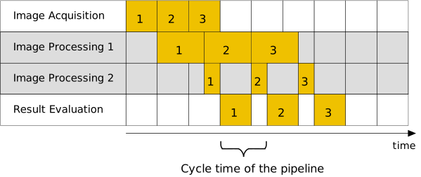
Figure 9 shows the scheduling diagram of a pipeline where the image processing stage was split into two stages. Here, it was not possible to split the image processing stage into two stages of equal size. Instead, the first part is three times larger than the second part. Compared to the simple pipeline described in Figure 6, the cycle time of the pipeline was only slightly reduced. The stage “Image Processing 1” is still significantly slower than the other stages and thus limits the throughput of the pipeline.
The second approach, parallel execution of the slowest stage on multiple threads, requires a little more implementation effort. However, it is usually easier to achieve a similar workload for the threads of this stage. Figure 10 shows such a pipeline, where the image processing stage runs on two threads in parallel.
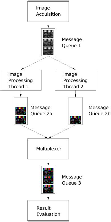
Depending on the image contents, the image processing task that was started last may finish before the task that was started first.
If it is required that the results appear in the same order the tasks were started, insert a a multiplexer after the parallel stage into the pipeline. A multiplexer guarantees that the tasks are returned in the same order they were started. It combines the output message queues of the parallel stage into one single message queue, which contains the tasks in correct order.
If the order of the results is irrelevant, for example, if the results are written into a database, no multiplexer is required. In these cases, the images can still be identified by their image ID.
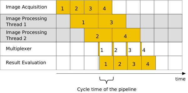
Figure 11 shows the scheduling diagram for the above discussed pipeline. The image processing of the second image starts while the first image is still being processed. Compared to Figure 6, the parallelization of the image processing stage (nearly) doubles the throughput of the pipeline.
Example implementation of the multithreaded pipeline🔗
The HDevelop example program hdevelop/System/Multithreading/pipeline_multiple_threads_per_stage.hdev shows an implementation of a pipeline where the image processing stage runs on multiple threads in parallel.
This is a pipeline similar to the one referred to in Figure 10 and Figure 11.
Note
In the following example, only the changes that are necessary to convert the simple pipeline as described in section Basic design of a pipeline into a pipeline that runs the image processing stage on multiple threads are described.
Multithreaded pipeline
In addition to the message queue that delivers the image processing results to the result evaluation stage, we need multiple message queues that connect the image processing stage with the multiplexer:
for I := 0 to NumImageProcessingThreads - 1 by 1
    create_message_queue (QueueImageProcessingResultsVector.at(I))
    set_message_queue_param (QueueImageProcessingResultsVector.at(I), \
                             'max_message_num', MessageQueueMaxMessageNum)
endfor
convert_vector_to_tuple (QueueImageProcessingResultsVector, \
                         QueuesImageProcessingResult)
Instead of starting only one thread for the image processing stage, we start multiple image processing threads as well as one multiplexer thread:
for I := 0 to NumImageProcessingThreads - 1 by 1
    par_start<ImageProcessingThreadVector.at(I)> : process_images (QueueOriginalImage, \
                                             NumAOPThreadsForImageProcessing, \
                                             TerminationKey, \
                                             QueueImageProcessingResultsVector.at(I))
endfor
convert_vector_to_tuple (ImageProcessingThreadVector, \
                         ImageProcessingThreads)
par_start<MultiplexerThread> : multiplexer (QueuesImageProcessingResult, \
                                            'image_id', TerminationKey, \
                                            QueueImageProcessingResult)
We wait for the additional threads to finish:
par_join ([AcquisitionThread,ImageProcessingThreads,MultiplexerThread, \
         ResultEvaluationThread])
To ensure a proper termination of the pipeline, we slightly modify the respective part of the procedure process_images.
In addition to enqueuing the termination message only to the output queue, we enqueue this message also to the input queue to inform the other threads that are running the procedure process_images as well:
get_message_param (MessageHandle, 'key_exists', TerminationKey, \
                    Terminate)
if (Terminate)
    enqueue_message_to_limited_queue (MessageHandle, QueueIn, 'wait')
    enqueue_message_to_limited_queue (MessageHandle, QueueOut, 'wait')
    break
endif
Finally, we implement the multiplexer.
The multiplexer ensures that the result evaluation stage receives the processing results in the correct sequential order.
Note that the messages do not need to be sorted or reordered.
As each input message queue is locally ordered, the multiplexer only has to look for the next message in the sequence by simultaneously monitoring the heads of all input message queues.
It determines the required order of the messages from the image ID, which was set in an increasing order by the image acquisition stage.
The basic functionality of the multiplexer is provided by the following lines of code:
NumInputQueues := |QueuesIn|
LastId := -1
Buffers := gen_tuple_const(NumInputQueues,-1)
Ids := gen_tuple_const(NumInputQueues,LastId)
while (1)
    for I := 0 to NumInputQueues - 1 by 1
            if (Buffers[I] == -1)
                dequeue_message (QueuesIn[I], [], [], MessageHandle)
                get_message_tuple (MessageHandle, SortIdKey, Id)
                Buffers[I] := MessageHandle
                Ids[I] := Id
            endif
            if (Buffers[I] != -1 and Ids[I] == LastId + 1)
                enqueue_message_to_limited_queue (Buffers[I], QueueOut, \
                                                  'wait')
                Buffers[I] := -1
                LastId := Ids[I]
            endif
    endfor
endwhile
The remainder of the multiplexer’s code, which can be found in the HDevelop example program hdevelop/System/Multithreading/pipeline_multiple_threads_per_stage.hdev, mainly deals with its termination if the pipeline is terminated and with the — unlikely — case that some messages are missing and therefore, there are gaps in the sequence of the image IDs.
Runtime behavior after speedup🔗
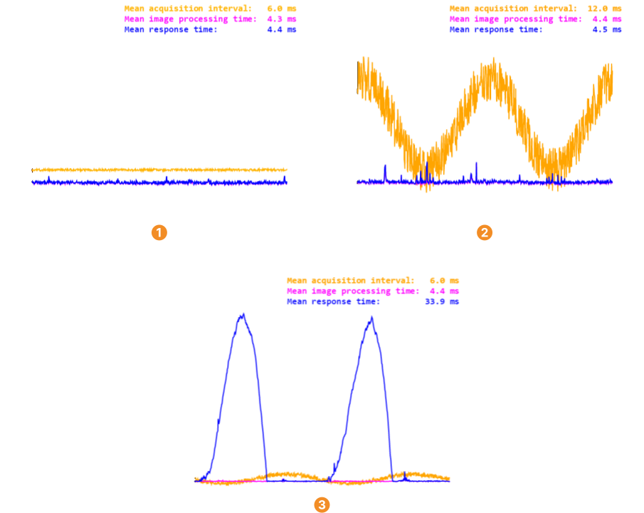
The runtime behavior of the pipeline with the image processing stage running on two threads is shown in Figure 12.
While it looks similar to that of the simple pipeline with only one thread per stage (see Figure 8), the acquisition interval may be significantly shorter.
Thus, the throughput of the system has been significantly increased.
Approximately constant acquisition interval
Varying acquisition interval
Varying acquisition interval leading to short-term peak loads
Enhancing the responsiveness🔗
The responsiveness can be enhanced using one of the following approaches:
- Producer consumer model, which is no parallelization concept in itself, but a method that can be used within any parallelization concept
- Specific parallelization scenarios
Producer consumer model🔗
The producer consumer model is not a parallelization concept or scenario but a method that can be used within various parallelization approaches.
In general, in this model one thread, the producer, provides some data, which one or several threads, the consumer(s), use for further processing.
A thread can be both producer and consumer, for example, within a pipeline, which consists of several producer consumer processes in row.
The communication between the producer and consumer threads is realized by message queues.
---
title: Enhancing the responsiveness using a producer consumer model
---
%%{ init: { 'flowchart': { 'curve': 'stepBefore' } } }%%
graph LR
    A["Producer"] -->|Message Queue| B["Consumer"]
The processing times are not always the same. Thus, if a producer thread acquires images and the consumer threads processes them, images can be lost if the processing threads are not ready to catch them in time. Images have to be buffered and special care has to be taken to avoid a buffer overflow. For a pipeline, this is demonstrated in Maximizing throughput via pipelining.
Further parallelization scenarios🔗
Different parallelization settings exist that enhance the responsiveness.
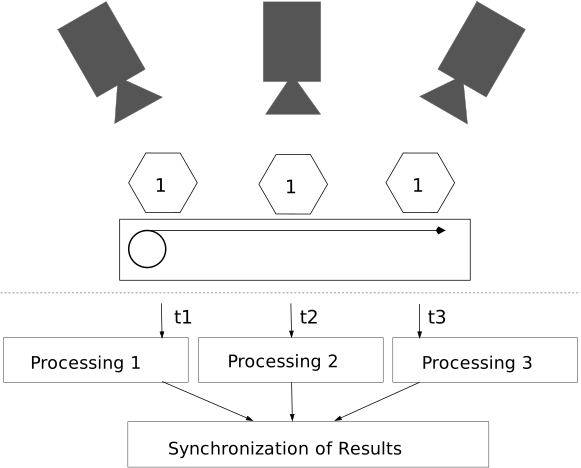
In Figure 13, an example setup is shown in which moving objects are viewed from different angles at different subsequent times.
Each image is processed in a separate thread.
The challenge is to synchronize the results after the processing.
Warning
In any case, synchronization is often challenging. Therefore, always try to reduce the need for synchronization as much as possible.
Other examples comprise the following:
- Scenarios in which input actions via keys, mouse clicks, IA, I/O etc. are expected
-
Scenarios in which a synchronization between the GUI and the processing steps is needed.
Note
This is not relevant in HDevelop, but when parallelizing within the language interfaces.