mean_curvature_flow🔗
Short description🔗
mean_curvature_flow — Apply the mean curvature flow to an image.
Signature🔗
mean_curvature_flow( image Image, out image ImageMCF, real Sigma, real Theta, integer Iterations )
Description🔗
The operator mean_curvature_flow applies the mean curvature
flow or intrinsic heat equation
to the gray value function \(u\) defined by the input image
Image at a time \(t_{0} = 0\). The discretized
equation is solved in Iterations time steps of length
Theta, so that the output image contains the gray value
function at the time Iterations \(\cdot\) Theta.
The mean curvature flow causes a smoothing of Image in the
direction of the edges in the image, i.e. along the contour lines of
\(u\), while perpendicular to the edge direction no smoothing is
performed and hence the boundaries of image objects are not
smoothed. To detect the image direction more robustly, in particular
on noisy input data, an additional isotropic smoothing step can
precede the computation of the gray value gradients. The parameter
Sigma determines the magnitude of the smoothing by means of
the standard deviation of a corresponding Gaussian convolution
kernel, as used in the operator isotropic_diffusion for
isotropic image smoothing.
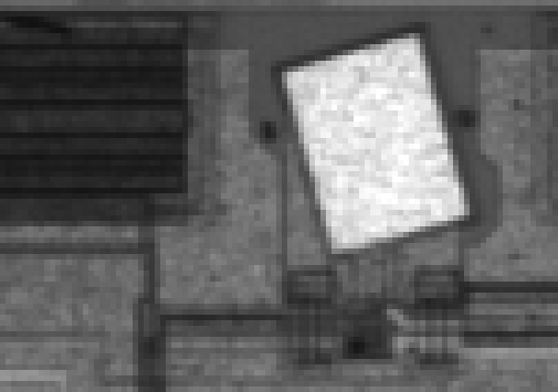
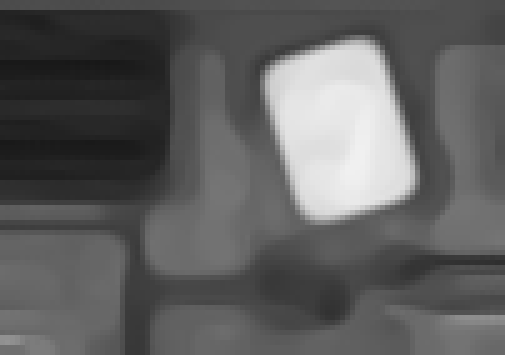
The following images show the effect of the parameters
Sigma, Theta, and Iterations. First, the
input image is shown together with the result that is achieved if
all parameters are set to their default values.
 |
 |
| (1) | (2) |
(1) Input image. (2) Result when using the default values.
In the following images, the results are shown that are achieved if one parameter is varied while setting the other two parameters to their default values.
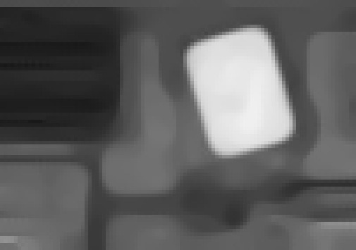
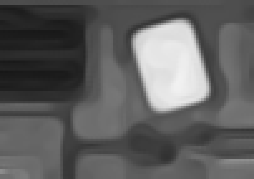
Sigma controls the amount of smoothing, prior to the
computation of the gray value gradient. Be careful with very large
values for Sigma, because they may lead to undesired effects.
 |
 |
 |
| (1) | (2) | (3) |
(1) Sigma = 0.0. (2) Sigma = 1.0. (3) Sigma = 10.0.
Theta controls the step size during the iterative smoothing
process. Larger values lead to a stronger smoothing.
 |
 |
 |
| (1) | (2) | (3) |
(1) Theta = 0.1. (2) Theta = 0.2. (3) Theta = 0.4.
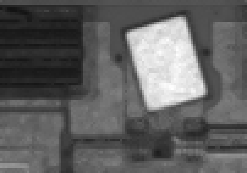
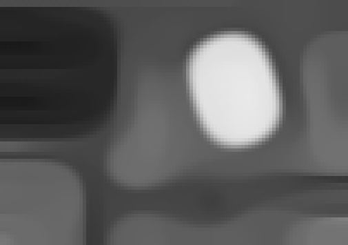
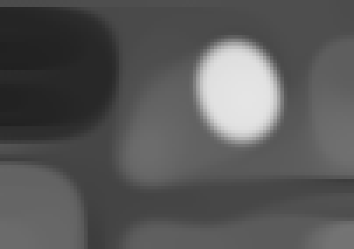
Iterations controls the number of iterations that are
performed. With an increasing number of iterations, the runtime
increases, as well. Furthermore, a large number of iterations may lead
to a loss of structure in the smoothed image.
 |
 |
 |
| (1) | (2) | (3) |
(1) Iterations = 1. (2) Iterations = 50. (3) Iterations = 100.
Attention🔗
Note that filter operators may return unexpected results if an image with a reduced domain is used as input. Please refer to the chapter Filters.
Execution information🔗
Execution information
-
Multithreading type: reentrant (runs in parallel with non-exclusive operators).
-
Multithreading scope: global (may be called from any thread).
-
Automatically parallelized on tuple level.
-
Automatically parallelized on channel level.
Parameters🔗
Image (input_object) (multichannel-)image(-array) → object (byte / uint2 / real)
Input image.
ImageMCF (output_object) image(-array) → object (byte / uint2 / real)
Output image.
Sigma (input_control) real → (real)
Smoothing parameter for derivative operator.
Default: 0.5
Suggested values: 0.0, 0.1, 0.5, 1.0
Restriction: Sigma >= 0
Theta (input_control) real → (real)
Time step.
Default: 0.5
Suggested values: 0.1, 0.2, 0.3, 0.4, 0.5
Restriction: 0 < Theta <= 0.5
Iterations (input_control) integer → (integer)
Number of iterations.
Default: 10
Suggested values: 1, 5, 10, 20, 50, 100, 500
Restriction: Iterations >= 1
References🔗
M. G. Crandall, P. Lions; ``Convergent Difference Schemes for Nonlinear Parabolic Equations and Mean Curvature Motion’‘; Numer. Math. 75 pp. 17-41; 1996.
G. Aubert, P. Kornprobst; ``Mathematical Problems in Image Processing’‘; Applied Mathematical Sciences 147; Springer, New York; 2002.
Module🔗
Foundation