Measure object basics🔗
The main idea behind the measure object is to extract edges that run approximately perpendicular to the line or arc of measurement. It is important to understand this process because you influence it with parameters both when creating the measure object and when applying it.
The next step is to specify the shape of the measuring ROI.
Please note that in contrast to other HALCON methods, measuring ROIs are not created using reduce_domain, but by specifying their dimensions when creating a measure object.
A measure object can be used to determine the position of straight edges that run approximately perpendicular to the given ROI.
1D edge extraction process🔗
HALCON determines the position of 1D edges by the following approach: First, equidistant lines of projection are constructed perpendicular to the line or arc of measurement (also called profile line) with a length equal to the width of the ROI (Figure 1).
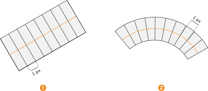
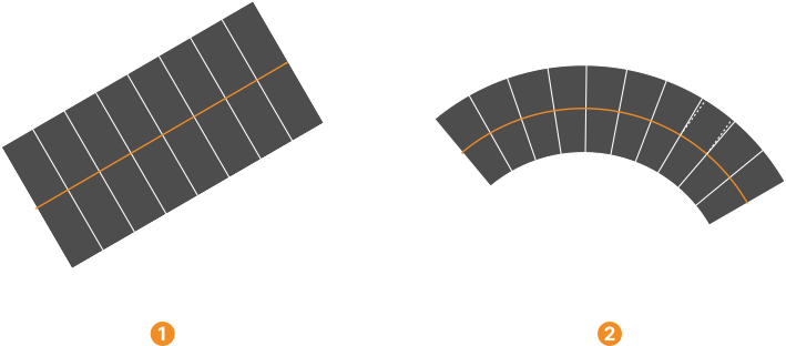
Then, the mean gray value along each line of projection is calculated.
The sequence of these mean values is called the profile.
If the lines of projection are not oriented horizontally or vertically, the pixel values along them must be interpolated.
You can select the interpolation mode with the parameter Interpolation of the operators for the creation of measure objects (for example, gen_measure_rectangle2).
If Interpolation = 'nearest_neighbor', the gray values in the measurement are obtained from the gray values of the closest pixel, that is, by constant interpolation.
This is the fastest method.
However, the geometric accuracy is slightly lower in this mode.
For Interpolation = 'bilinear', bilinear interpolation is used, while for Interpolation = 'bicubic', bicubic interpolation is used.
The bicubic interpolation yields the most accurate results.
However, it is the slowest method.
The length of the lines of projection, that is, the width of the ROI, defines the degree of averaging in the direction perpendicular to the profile line. The thick lines in and show the profiles for the two ROIs displayed in and . It can be seen that the profile that corresponds to the wider ROI is less noisy. Therefore, as long as the edges run approximately perpendicular to the profile line, the ROI should be chosen as wide as possible. If the edges do not run perpendicular to the profile line, the width of the ROI must be chosen smaller to allow the detection of edges. Note that in this case, the profile will contain more noise. Consequently, the edges will be determined less accurate.
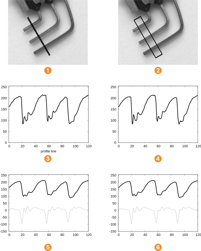
ROI of Width=2
ROI of Width=20
Width=2, no smoothing
Width=20, no smoothing
Width=2, Sigma=1.1
Width=20, Sigma=1.1
The profile is then smoothed with a Gaussian smoothing filter (see the thick lines in
and
), whose standard deviation is specified with the parameter Sigma of the measuring operators (for example, measure_pairs).
Now, the first derivative of the smoothed profile is calculated (thin lines in
).
Note that the amplitude of the derivative is scaled with a factor \(\sqrt{2\pi}\) · Sigma.
The subpixel precise positions of all local extrema of the first derivative are edge candidates.
In
, these edge candidates are indicated by vectors pointing from the respective position of the derivative (thin line) to the smoothed gray value profile (thick line).
Only those edge candidates that have an absolute value of the first derivative larger than a given Threshold (another parameter of the measuring operators) are considered as edges in the image (see
).
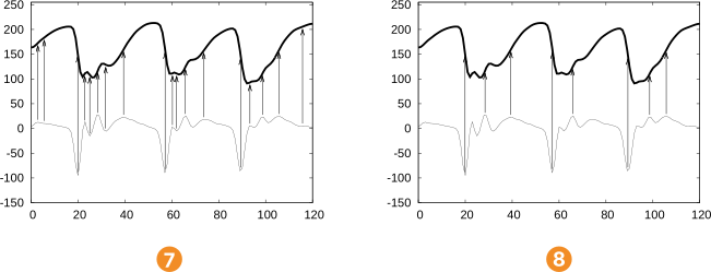
Sigma = 1.1. X-axis corresponds to the position on the profile line, Y-axis corresponds to the gray value.
edge candidate positions
edge positions
For each edge, the position of its intersection with the profile line is returned. Figure 4 shows the detected edges, displayed by straight lines with a length similar to the width of the ROI.
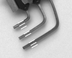
Threshold of 20.Note that the above described approach for the extraction of 1D edges from a profile differs significantly from the 2D edge extraction performed, for example, with the operator edges_sub_pix (compare Figure 5).
In the case of the 1D edge extraction, only the positions of the intersections of the edges with the profile line are determined as described above whereas the 2D edge extraction returns the complete edges as contours.
If the edges are straight and run approximately perpendicular to the profile line, the results of the 1D edge extraction are similar to the intersection of the 2D edges with the profile line.
The more the edges are curved or not perpendicular to the profile line, the more different the results of the two approaches will be.
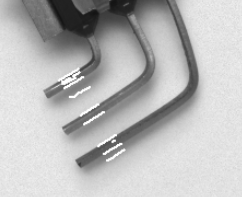
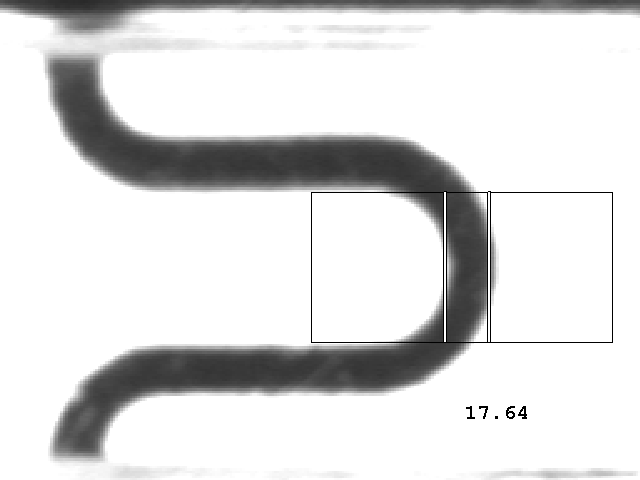
Keep in mind that measure objects are designed to measure the position of straight edges that run approximately perpendicular to the profile line. This means that measure objects are not suited to measuring the position of, for example, curved edges. In those cases, the measure position will typically not coincide with the intersection of the gray value edge with the profile line. An example for such a case is given in Figure 6. Here, the edges are curved, which leads to wrong measurement results. This effect will be reduced if the width of the ROI is chosen smaller.
Measure object creation🔗
Measure objects can be created with two different shapes: Rotated rectangles and circular arcs.
They are created with the operators gen_measure_rectangle2 or gen_measure_arc.
To create a rectangular measure object, you use the operator gen_measure_rectangle2:
gen_measure_rectangle2 (Row, Column, Phi, Length1, Length2, Width, Height, Interpolation, MeasureHandle)
A rotated rectangle is defined by its center (Row, Column), its orientation Phi, and its half edge lengths Length1 and Length2 (see
in Figure 7).
The parameter Phi is given in radians in mathematically positive sense.
All the other parameters are given in pixels.
To create a circular measure object, you use the operator gen_measure_arc:
gen_measure_arc (CenterRow, CenterCol, Radius, AngleStart, AngleExtent, AnnulusRadius, Width, Height, Interpolation, MeasureHandle)


The circular arc is defined by the following parameters (see
in Figure 7): The position and size are defined by the center (CenterRow, CenterColumn) and the radius (Radius).
The segment of the circle is defined by its start angle (AngleStart) and the angular extent (AngleExtent).
The width of the circular ROI is defined by the annulus radius (AnnulusRadius).
Again, all parameters are given in pixels, except for the angles (AngleStart and AngleExtent), which are given in radians in mathematically positive sense.
The first parameters of both operators for the creation of measure objects define the position, size, and orientation of the respective ROI.
The parameters Width and Height are the size of the images, on which the measure can be applied.
The parameter Interpolation sets the interpolation mode.
Note that when using interpolation, not only the ROI but additionally the margin around the ROI must fit into the image.
The width of the margin (in all four directions) has to be at least 1 pixel for a bilinear interpolation and two pixels for a bicubic interpolation.
For lines of projection that do not fulfill this condition, no result is obtained.
The result for both operators is a handle for the newly created measure object (MeasureHandle), which can then be used to specify the measure object, for example, in calls to the operator measure_pos.
Note that if you use HALCON’s C++ interface and call the operator via the classes HMeasureX or HMeasure, no handle is returned because the instance of the class itself acts as your handle.