2D measuring🔗
More Info
Learn about 2D measuring and many other topics in interactive online courses at our MVTec Academy.
Measuring in images consists of the extraction of specific features of objects. 2D features that are often extracted comprise:
- The area of an object, like the number of pixels representing the object.
- The orientation of an object.
- The angle between objects or segments of objects,
- The position of an object.
- The dimension of an object: diameter, width, height, or the distance between objects or parts of objects.
- The number of objects.
To extract the features, several tools are available. Which tool to choose depends on the goal of the measuring task,the required accuracy, and the way the object is represented in the image.
In general, the extraction of elements from an image is preceded by the image acquisition. A good measurement result highly depends on the quality of the image.
More Info
The chapter “Appendix C, Object Appearance” in the Solution Guide II-A – Image Acquisition discusses how to obtain a good quality image.
Region processing🔗
For objects or object parts that are represented by regions of similar gray value, color, or texture, blob analysis is a fast and simple way to extract objects and their features. The image is segmented into so-called blobs, which are regions in the image that comprise a specific range or behavior of pixel values (see Blob analysis).
The blob analysis consists of different essential steps, not necessarily applied in that order:
- The preprocessing.
- The segmentation of the image into regions.
- The modification of the regions.
- The extraction of the region features that are searched for.
Preprocessing images or regions🔗
A preprocessing is recommended if the conditions during the image acquisition are not ideal, for example the image is noisy, cluttered, or the object is disturbed or overlapped by objects of small extent so that small spots or thin lines prevent the actual object of interest from being described by a homogeneous region.
Often applied preprocessing steps comprise the elimination of noise using the operator mean_image or binomial_filter, and the suppression of small spots or thin lines with the operator median_image.
Further operators are:
gray_opening_shapegray_closing_shapesmooth_image, for smoothing the imageanisotropic_diffusion, for smoothing the image but preserve the edgesfill_up, for filling holes
Morphological operators modify regions to suppress small areas, regions of a given orientation, or regions that are close to other regions.
opening_circleandopening_rectangle1suppress noise.closing_circleandclosing_rectangle1fill gaps.
When having an inhomogeneous background, a shading correction is suitable to compensate the influence of the background, where a reference image of the background without the object to measure is taken and subtracted from the images containing the object using sub_image.
Segmenting images into regions🔗
After the preprocessing the image must be segmented into suitable regions that represent the objects of interest. Several kinds of threshold operators are available that segment a gray-value image or a single channel of a multichannel image according to its gray value distribution.
Common threshold operators are:
When choosing a threshold manually, it may be helpful to get information about the gray value distribution of the image. Suitable operators are:
Additionally, you can use the online Gray Histogram inspection to interactively search for a suitable threshold.
After segmenting the image with a threshold operator, the image parts of interest are available as one region.
To split this region into several regions, one region for every connected component, the operator connection must be applied.
For objects with a honeycomb structure, watershed operators are better suited than a threshold operator, as they segment the image based on the topology instead of the distribution of the gray values.
If you want to obtain regions having the same intensity, apply regiongrowing. For both operators a preprocessing using a low pass filter like binomial_filter is recommended.
Selecting and modifying regions🔗
After segmenting the image into a set of regions, regions having specific features can be selected using operators like select_shape or select_gray.
Common features are, for example, a specific area range, a certain shape, or a specific gray value.
For the list of all features that can be used for the selection, see the reference entry of the select_shape operator, for example.
In many cases, a modification of the regions is necessary.
For example, small gaps or small connections can be eliminated by a morphological operator like opening_circle or dilation_rectangle1.
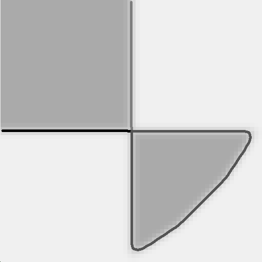
Different regions can be combined by the set-theoretical operators shown in Figure 1.
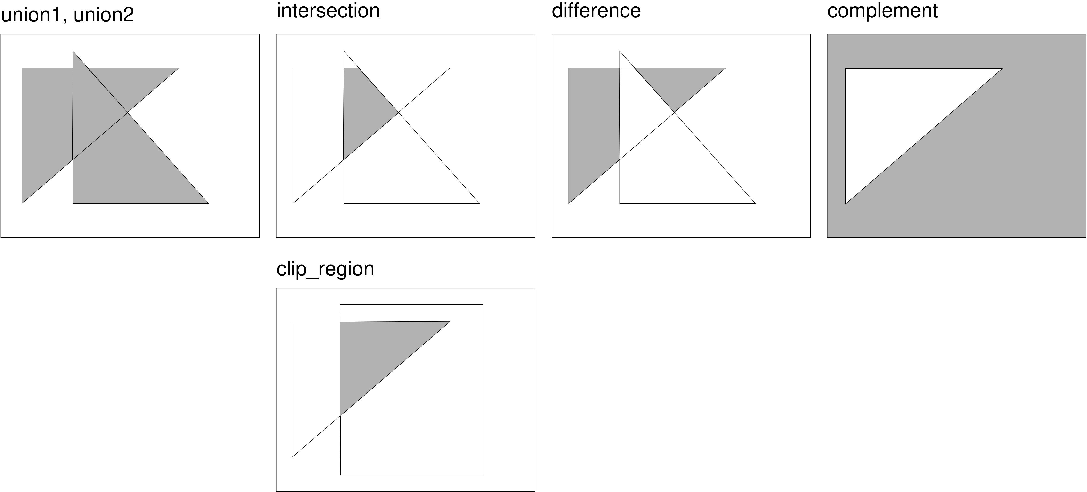
-
intersectionreturns the intersection of regions. -
differencesubtracts the overlapping part of two regions from the first region. -
complementobtains the complement of a region.
If you need the intersection of regions with a rectangle,for example, created by gen_rectangle1, you should use clip_region. It works similar to intersection but is more efficient.
Another way of modifying a region is to transform it, in particular to approximate it by a specific shape using the operator shape_trans.
This approach is suited if the features of the approximating shape describe the features you try to obtain.
For example, if you search for the maximum width of an object, you can approximate the shape by its smallest enclosing rectangle or circle and extract its width or radius.
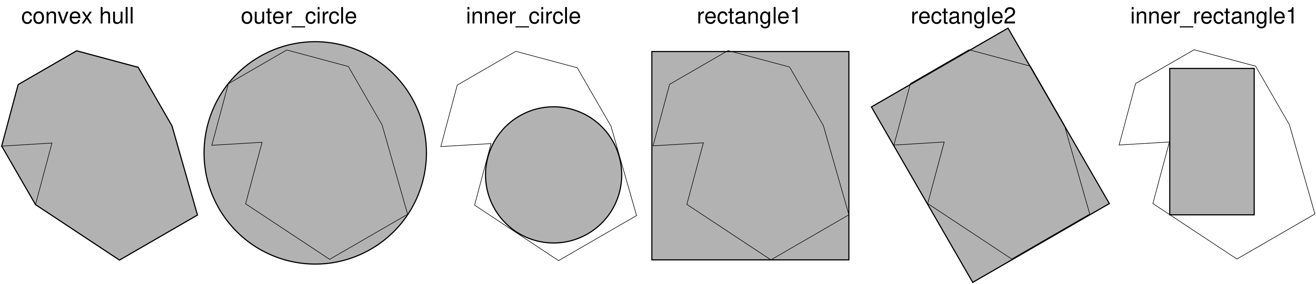
-
convex: convex hull -
outer_circle: smallest enclosing circle -
inner_circle: largest circle fitting into the region -
rectangle1: smallest enclosing rectangle parallel to the coordinate axis -
rectangle2: smallest enclosing rectangle with arbitrary orientation -
inner_rectangle1: largest rectangle parallel to the coordinate axis that fits completely into the region -
ellipse: ellipse with the same moments as the input region -
inner_center: point on the skeleton of the input region having the smallest distance to the center of gravity of the input region
Extracting features🔗
Having obtained the region that represents the object to measure, the features of the object, the actual measurement results, can be extracted.
Several operators are provided to compute features like the area, position, orientation, or dimension of a region. Some of them can be used as alternatives to the shape transformations described in the preceding section.
Common operators are:
-
area_centercomputes the area and the position of the center of an arbitrarily shaped region. -
smallest_rectangle1andsmallest_rectangle2compute the smallest enclosing rectangle. In particular,smallest_rectangle1computes the corner coordinates for the smallest surrounding rectangle being parallel to the image coordinate axes, andsmallest_rectangle2computes the radii (half lengths), position, and orientation of the smallest enclosing rectangle with arbitrary orientation. -
inner_rectangle1computes the corner coordinates for the largest rectangle parallel to the coordinate axes that fits completely into the region. -
inner_circledetermines the radius and position of the largest circle fitting into the region. -
diameter_regionobtains the maximum distance between two boundary points of a region. -
orientation_regionis used to get the orientation of a region.
orientation_region and smallest_rectangle2 both compute the orientation of the object, but the results of both can differ, depending on the shape of the object.
If you prefer to work with contour processing instead of region processing, and a pixel-precise measuring is sufficient, you can also start with region processing and at any time convert the regions into contours with gen_contour_region_xld.
Contour processing🔗
Contour processing is suitable for high precision measuring, for objects that are not represented as homogeneous regions in the image but by clear gray value or color transitions (edges), or for object parts that are not bordered by a closed contour.
Creating contours🔗
Contour processing starts with the creation of contours. The common way to obtain contours is to extract edges. Edges are transitions between dark and light areas in an image and can be mathematically determined by computing the image gradient, which can also be represented as edge amplitude and edge direction. By selecting pixels with a high edge amplitude or a specific edge direction, contours between areas can be extracted. This can be done in various ways and with varying precision.
Pixel-precise edges and lines🔗
If a pixel-precise edge extraction is sufficient, an edge filter can be applied. It leads to one or two edge images, for which the edge regions can be extracted by selecting the pixels with a given minimum edge amplitude using a threshold operator.
-
To get edges with a thickness of one pixel, the obtained regions have to be thinned, for example by using the operator
skeleton. -
Common pixel-precise edge filters are the operator
sobel_amp, which is fast, andedges_image, which is not that fast but already includes a hysteresis threshold and a thinning and leads to more accurate results. -
edges_imageand also its equivalent for color images,edges_color, can also be applied with the parameterFilterset tosobel_fast. Then, it is fast as well, but this parameter is recommended only for images with little noise or texture and sharp edges. -
Besides edges, you can also extract lines that are built by thin structures on a contrasting background. In contrast to edges or the XLD lines that are obtained by a line fitting, they have a certain, not necessarily constant, width. A common filter for these lines is
bandpass_image, which is again applied in combination with a threshold and a thinning. -
For edge filters, after applying the filter, threshold, and thinning, the result typically is transformed into XLD contours. With this approach, a broad range of further processing methods is available. For the transformation of the thinned edge regions into contours, for example, the operator
gen_contours_skeleton_xldis provided.
Subpixel-precise edges and lines🔗
If a pixel-precise extraction is not sufficient, operators for the subpixel-precise edge and line extraction can be applied. These immediately return XLD contours.
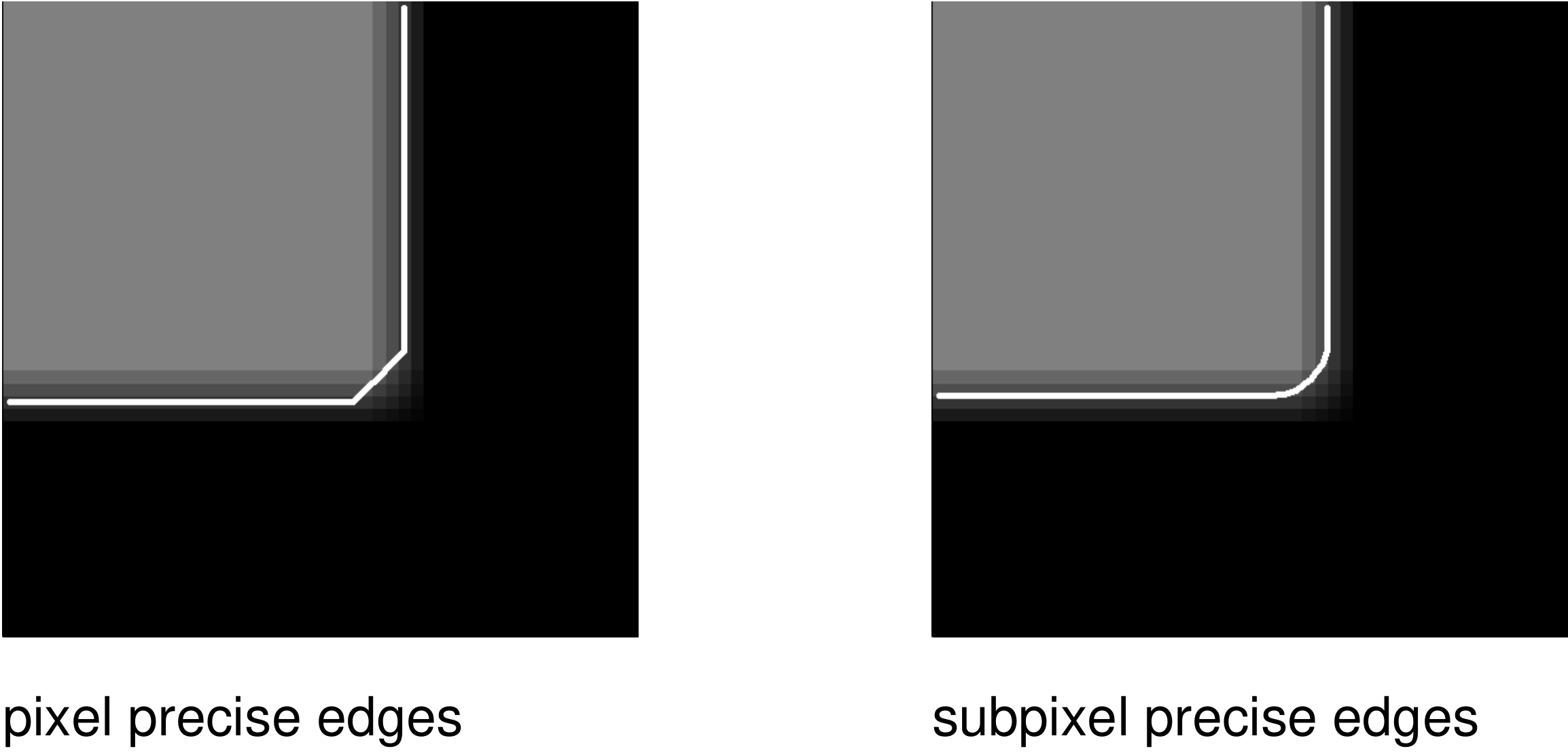
Common operators to extract subpixel-precise edges are:
edges_sub_pixfor the general edge extraction.edges_color_sub_pixfor extracting edges in color images.zero_crossing_sub_pixfor extracting zero crossings in an image, or respectively, to extract edges in Laplace-filtered images.
Common operators for the extraction of subpixel-precise lines, thin linear structures with a certain (not necessarily constant) width, are:
lines_gaussfor the general line extraction.lines_facetfor extracting lines using a facet model.lines_colorfor extracting lines in color images.
Speeding up the contour extraction🔗
To speed up the subpixel-precise edge extraction, it is recommended to apply it only to a small region of interest (ROI).
To obtain a suitable ROI you can, determine the region enclosed by the contour with a thresholding by using fast_threshold.
The returned region then must be reduced to its boundary by the operator boundary and possibly clipped by clip_region_rel.
With a morphological operator, for example, dilation_circle, the region is expanded by a small amount
The image is reduced to the returned region by reduce_domain.
The reduced image is used as an ROI.
The ROI builds the search space for the subpixel-precise edge extraction.
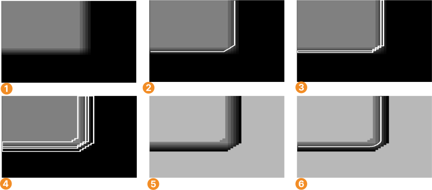
Original image
Pixel-precise edge extraction
Boundary for the edge region
Dilation of the region
Reduced domain (ROI)
Subpixel-precise edge extraction within the ROI
Subpixel-precise thresholding🔗
Another fast way to extract contours is provided by the subpixel-precise thresholding using the operator threshold_sub_pix, which can be applied in real time to a whole image.
It is a thresholding operator similar to the ones used for the region processing, but in contrast to them it does not result in a closed region but in subpixel-precise contours describing the border or parts of a border of the region.
In contrast to the threshold operators introduced for the region processing the returned contours need not be closed, multiple contours can be obtained for the same region, and junctions between contours are possible.
Like for the thresholding operators used for a region processing, you can search for a suitable threshold using, the online Gray Histogram inspection, or obtain information about the gray value distribution of the image by the operators:
Getting relevant contours🔗
If the creation of the contours led to more contours than needed for the further processing, there are means to reduce the set of extracted contours to a set of contours relevant for the specific measuring task.
Suppressing irrelevant contours🔗
You can suppress irrelevant contours by selecting only those contours fulfilling specific constraints.
For example, the operator select_shape_xld can be used to select closed contours with a specific shape feature concerning, like the contour’s convexity, circularity, or area. Almost 30 different shape features are available, which are listed in About regions.
A similar operator for the selection of specific contours is select_contours_xld.
It can be used to select open and closed contours according to typical line features like length, curvature, or direction.
The operator select_xld_point can be used in combination with mouse functions to interactively select contours.
Combining contours🔗
When having several contours that approximate the same object part, the number of segments can further be reduced by a contour merging.
Suitable operators are:
-
The contours lie approximately on the same line use (
union_collinear_contours_xld). -
The contours lie on the same circle use
union_cocircular_contours_xld. -
The contours are adjacent use (
union_adjacent_contours_xld). -
The contours lie are cotangential use (
union_cotangential_contours_xld).
For closed contours or polygons, you can also use set-theoretical operators to combine the enclosed regions of different closed contours or polygons. This is similar to the approach for the region processing.
Available operators are:
-
intersection_closed_contours_xldandintersection_closed_polygons_xldfor the calculation of the intersection of regions that are enclosed by closed contours or polygons. -
difference_closed_contours_xldanddifference_closed_polygons_xldfor the calculation of the difference between regions that are enclosed by closed contours or polygons. -
symm_difference_closed_contours_xldandsymm_difference_closed_polygons_xldfor the calculation of the symmetric difference between regions that are enclosed by closed contours or polygons. -
union2_closed_contours_xldandunion2_closed_polygons_xldfor merging regions that are enclosed by closed contours or polygons.
Simplifying contours🔗
Contours can be simplified by directly transforming them into shape primitives, which is similar to the approach for the region processing but now for on contours instead of regions.
With shape_trans_xld you can transform a contour into:
- The smallest enclosing circle.
- The ellipse having the same moments.
- The convex hull.
- The smallest enclosing rectangle either parallel to the coordinate axis or with arbitrary orientation.
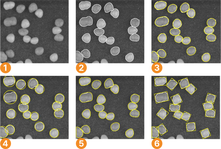
Original image
Extracted contours after suppression of irrelevant contours
Contours transformed into ellipses with the same moments
Contours transformed into their smallest enclosing circles
Contours transformed into their convex hulls
Contours transformed into their smallest enclosing rectangles with arbitrary orientation
Segmenting contours🔗
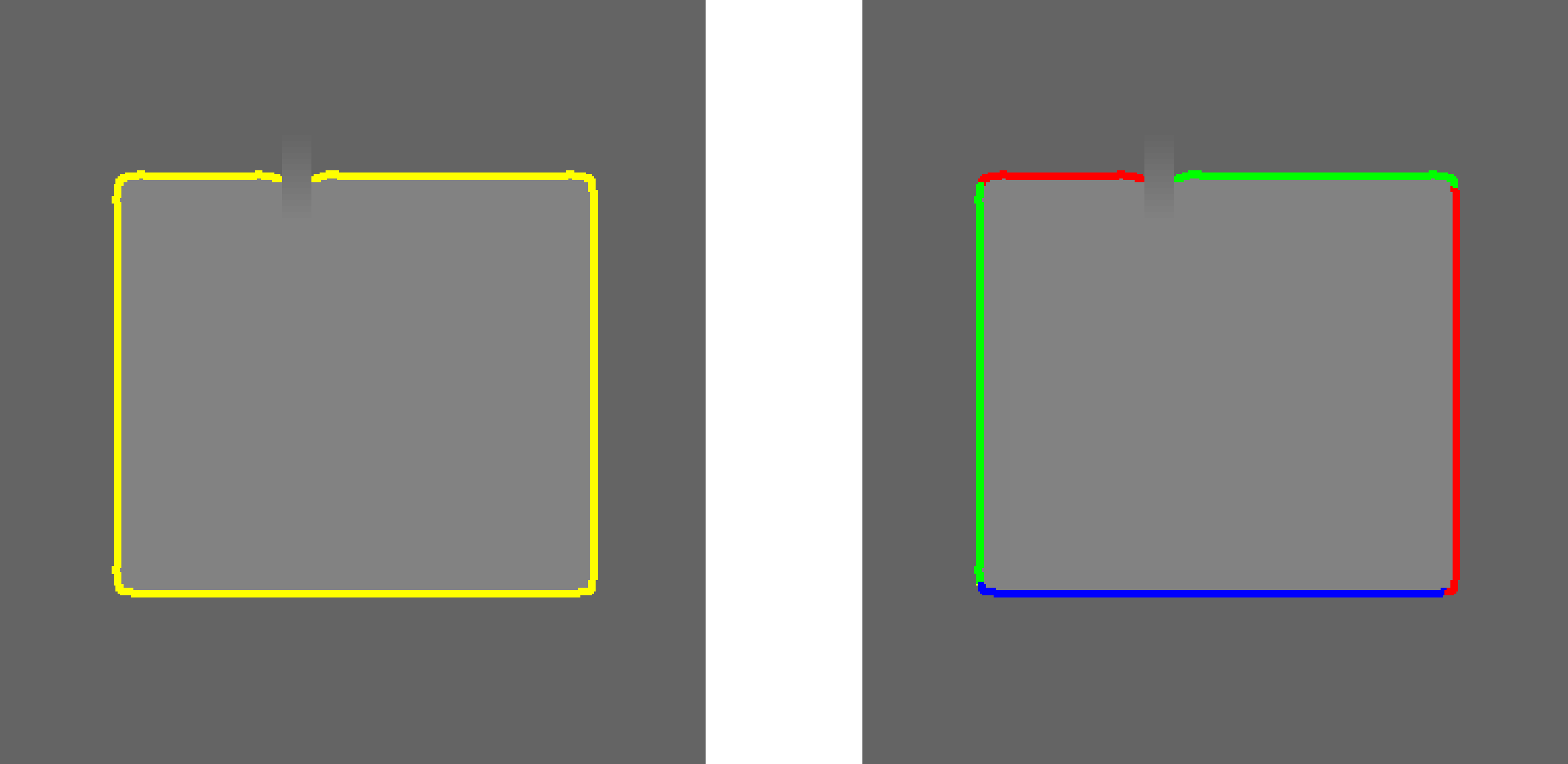
A segmentation of the contour into less complex contours helps to make the investigation of the object easier, as each segment can be measured individually.
For the measuring, primitive shapes like lines or circles are fitted to the segments and their parameters, for example, the diameter of a circle or the length of a line, can be obtained. Dependent on the chosen parameters, a contour can be segmented into linear segments, linear and circular segments, or linear and elliptic segments.
Available shape primitives for a shape fitting include lines, circles, ellipses, and rectangles. For the contour segmentation the operator segment_contours_xld can be applied.
The information by which shape each individual segment is approximated is stored in the attribute cont_approx.
If you need only straight line segments, you can alternatively use the operator gen_polygons_xld instead.
To get the individual line segments of the polygon, apply the operator split_contours_xld.
Extracting features of contour segments by approximating them by known shapes🔗
The common step after the selection and possibly a segmentation is to fit shape primitives to the contours or contour segments to get their specific shape parameters.
The available shape primitives are lines, circles, ellipses, and rectangles. The obtained features may be, for example, the end points of the lines or the centers and radii of the circles.
For each segment the value of cont_approx, the shape of the segment, can be queried with the operator get_contour_global_attrib_xld.
Depending on its value, the best-suited shape primitive can be fitted into the contour segment using the corresponding fitting approach:
-
Use (
cont_approx = -1)fit_line_contour_xldfor linear segments to get the parameters of each line segment, for example, the coordinates for both end points. -
Use (
cont_approx = 1) :fit_circle_contour_xldfor circular arcs. -
Use (
cont_approx = 0) :fit_ellipse_contour_xldfor elliptic arcs. -
Rectangles consist either of a pure, unsegmented, contour or of linear contours that have been merged, for example, by
union_adjacent_contours_xld. For them, the operatorfit_rectangle2_contour_xldis provided.
With the obtained parameters the corresponding contour can be generated for a visualization or a further processing. Lines can be generated with gen_contour_polygon_xld, circles with gen_circle_contour_xld, ellipses with gen_ellipse_contour_xld, and rectangles with gen_rectangle2_contour_xld. For the visualization, common visualization operators like dev_display are used.
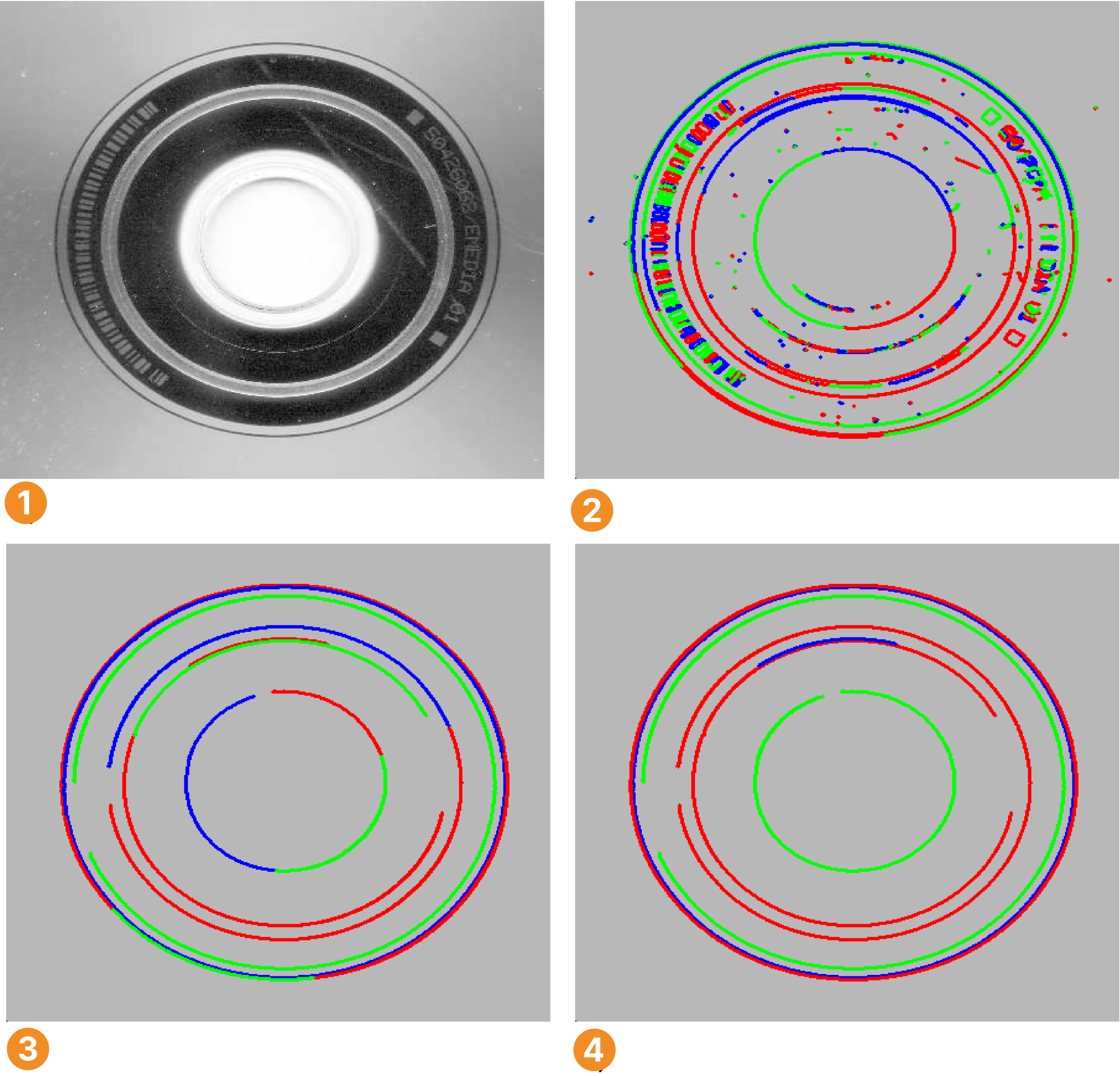
Original image
Contours after suppression of irrelevant contours
Circles fitted into the contours
Visualization of radius R for each circle
Extracting features of contours without knowing their shapes🔗
If the object to investigate cannot be described by a predefined shape primitive, HALCON provides several operators that compute general features of contours.
Similar to the operators used for the feature extraction within a region processing, features like orientation or area can be queried.
Common operators used for 2D measuring with contours are:
-
area_center_xld: area and center of gravity for the region enclosed by the contour or polygon, and the order of the points along the boundary. -
diameter_xld: the coordinates of the two extreme points of the contour having the maximum distance, and the distance between them. -
elliptic_axis_xld: the two radii and the orientation of the ellipse having the same orientation and aspect ratio as the contour. -
length_xld: length of the contour or polygon. -
orientation_xld: orientation of the contour. -
smallest_circle_xld: center position and radius of the smallest enclosing circle. -
smallest_rectangle1_xld: coordinates of the corners describing the smallest enclosing rectangle that is parallel to the coordinate axis. -
smallest_rectangle2_xld: center position, orientation, and the two radii (half lengths) of the smallest enclosing rectangle with arbitrary orientation.
Some of the operators only work on contours that have no self intersections.
Self intersections are not always obvious as they can occur due to internal calculations of an operator, for example, if an open contour is closed for the needed operation.
To check if a contour intersects itself you can apply the operator test_self_intersection_xld.
If you face problems because of self intersections, you can also use the corresponding point-based operators.
The available operators are:
About areas🔗
The area of an object is in most cases obtained by the operator area_center.
If a subpixel-precise measuring requires contour processing, you can use the corresponding operator area_center_xld or area_center_points_xld instead.
Be aware that when computing the area of a region, possible holes in the region are considered, whereas when computing the area of a contour, the whole area enclosed by the contour is obtained.
In the latter case, you therefore have to extract also the contours of the holes, get their areas, and subtract them from the area enclosed by the outer contour. The operator area_holes calculates the area of the holes in the input regions.
2D metrology🔗
If you want to measure objects that are represented by simple shapes like circles, ellipses, rectangles, or lines, and you have approximate knowledge about their positions, orientations, and dimensions, you can use 2D metrology to determine the exact shape parameters. In particular, the values of the initial shape parameters are refined by a measurement that is based on the exact location of edges within so-called measure regions. These are rectangular regions that are evenly distributed along the boundaries of the approximately known shapes.
The example program hdevelop\2D-Metrology\apply_metrology_model shows the basic steps of 2D metrology:
-
A metrology model must be created using
create_metrology_model. In this model, all needed information related to the objects to measure will be stored. -
To enable an efficient measurement, the size of the image in which the measurements will be performed should be added to the model using the operator
set_metrology_model_image_size. -
The approximate values for the shapes of the objects in the image and some parameters that control the measurement must be added.
For each shape, depending on its geometric type, the following operators are used:
-
add_metrology_object_circle_measureadds parameters of one or more circle(s), the coordinates of the center point and the radius. -
add_metrology_object_ellipse_measureadds parameters of one or more ellipse(s), the coordinates of the center point, the orientation of the main axis, and the size of the smaller and the larger half axis. -
add_metrology_object_line_measureadds parameters of one or more line(s), the coordinates of the start and end point. -
add_metrology_object_rectangle2_measureadds parameters of one or more rectangle(s), the coordinates of the center point, the orientation of the main axis, and the size of the smaller and the larger half axis. -
add_metrology_object_genericadds parameters of circles, ellipses, lines, and/or rectangles. Note that you can change several parameters that control the measurement with the operatorset_metrology_object_param.
In the example program, values for a rectangular and a circular object are added.
The actual measurement in the image is performed with the operator apply_metrology_model.
The refined shape parameters that result from the measurement can be accessed from the metrology model with the operator get_metrology_object_result.
To inspect the contours that have been added to the metrology model, use get_metrology_object_model_contour.
To access the measure regions, which may be helpful when adjusting the parameters that control the measurement, you can call the operator get_metrology_object_measures.
Aligning the metrology model based on different methods🔗
The example program hdevelop/Applications/Measuring-2D/measure_stamping_part shows how the metrology model can be aligned, for example, if the object’s position varies from image to image.
- Shape-based matching
- To find the objects to be measured in a new image, create and train a shape model.
For more information about shape-based matching and its parameters, see Shape-based matching and
set_generic_shape_model_param. - Region processing
- The alignment can also be performed via region processing. In this case, we use
area_centerandorientation_regionto determine the reference position of the segmented reference object.
In the online phase, first segment the object the same way as in the reference image and determine its position and orientation. If the reference system of the metrology model has been set, the result can directly be used for the alignment withalign_metrology_model. Finally, you can perform the actual measurement withapply_metrology_model. - Rigid transformation from point correspondences
-
If it is possible to robustly detect correlated reference points in the reference image as well as in the online images, it is possible to calculate a rigid transformation from these point correspondences and use it for alignment.
-
First, extract the reference points for the alignment. In the example, the procedure
extract_reference_pointsis used for this purpose. In this case, no reference system has to be set. In the online phase, extract the reference points and determine the rigid transformation parameters using the operatorsvector_to_rigidandhom_mat2d_to_affine_par. You have to take care that corresponding points have the same indices inRowReference,ColumnReference,RowExtracted, andColumnExtracted. The results are then used for the alignment withalign_metrology_model. Finally, you can perform the actual measurement withapply_metrology_model. - Querying Results
-
The example also shows how to query results.
-
The edge points that were actually used to fit the geometric forms can be visualized with
get_metrology_object_result.
Geometric operations🔗
HALCON provides a selection of operators for geometric operations to calculate the relation between elements like points, lines, line segments, contours, or regions.
Points can be determined by several point operators, for example, points_foerstner, or by the intersection of lines.
The relations between the individual elements can be calculated by several operators. Most of the operators are constructed to calculate the distance relation between the elements.
The operators for the distance relations are:
| Point | Line | Line Segment | Contour | Region | |
|---|---|---|---|---|---|
| Point | distance_pp |
distance_pl |
distance_ps |
distance_pc |
distance_pr |
| Line | distance_pl |
— | distance_sl |
distance_lc |
distance_lr |
| Line Segment | distance_ps |
distance_sl |
distance_ss |
distance_sc |
distance_sr |
| Contour | distance_pc |
distance_lc |
distance_sc |
distance_cc, distance_cc_min |
— |
| Region | distance_pr |
distance_lr |
distance_sr |
— | distance_rr_min, distance_rr_min_dil |
Further operators for geometric operations can be used to calculate the following:
- Angle between two lines:
angle_ll - Angle between a line and the vertical axis:
angle_lx - Point on an ellipse corresponding to a specific angle:
get_points_ellipse - Intersection of two lines:
intersection_lines - Projection of a point onto a line:
projection_pl
More Info
Learn about 2D measuring and many other topics in interactive online courses at our MVTec Academy.