Example cases for 2D measuring🔗
Rotating image and region🔗
For many measuring tasks, it is useful to align the object of interest parallel to the coordinate axis of the image.
If the object cannot be aligned already at the image acquisition, the image or the extracted regions must be rotated by image processing.
The example program %HALCONEXAMPLES%\solution_guide\2d_measuring\measure_screw measures different dimension-related features of a screw.
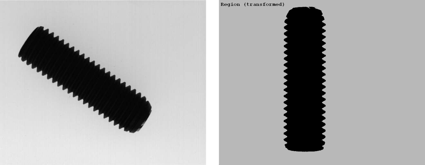
Steps within the example:
-
Determine parameters for the rotation.
Before applying a 2D transformation, the parameters for the transformation must be determined. Here, the region of the object is extracted usingthreshold (Image, Region, 0, 100) orientation_region (Region, OrientationRegion) area_center (Region, Area, RowCenter, ColumnCenter)thresholdand the orientation of the region is determined viaorientation_region. The orientation intended for the following measuring is 90°.As center for the rotation we choose the center position of the region, which we obtain with
area_center. Because of the approximately symmetrical shape of the screw, the screw can be twisted by 180°, but for the described task it is not important at which side of the screw we start to measure. -
Create the homogeneous transformation matrix
The operatorvector_angle_to_rigid (RowCenter, ColumnCenter, OrientationRegion, \ RowCenter, ColumnCenter, rad(90), HomMat2DRotate)vector_angle_to_rigidcreates a homogeneous transformation matrix for a simultaneous rotation and translation. Here, only a rotation is applied, meaning the center point is the same for the original and the transformed region and only the angle is changing from the original orientation to the vertical direction.An additional translation is recommended, for example, if similar objects in several images have to be placed in the same position so that a direct comparison between them is possible. Another need for a translation occurs if the object or parts of it moved out of the image because of the rotation.
Alternatively, you can also create a homogeneous transformation matrix for the identical 2D transformation by
hom_mat2d_identity, and add a rotation and a translation to it byhom_mat2d_rotateandhom_mat2d_translate, respectively.A scaling can also be added to the homogeneous transformation matrix by
hom_mat2d_scale, but a scaling significantly influences the absolute values obtained by the measuring. To compensate this, you can afterwards transform the measurement results back to the original dimension by applying the inverse transformation matrix to them. -
Transform region.
The actual transformation of the region is realized by the operatorvector_angle_to_rigid (RowCenter, ColumnCenter, OrientationRegion, \ RowCenter, ColumnCenter, rad(90), HomMat2DRotate)affine_trans_region(see Figure 1). The rotated region is now used for the measuring task described in the next section.
Measuring the width of screw thread🔗
The first measuring approach of the example program %HALCONEXAMPLES%\solution_guide\2d_measuring\measure_screw measures the minimum, maximum, and mean width of a screw thread.
For this, we use the vertical region of the screw obtained before and measure the difference between the column coordinates of the region’s border in each row.
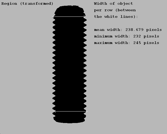
Steps within the example:
-
Get object width for each row.
The operatorclosing_circle (RegionAffineTrans, RegionToProcess, 4.5) get_region_runs (RegionToProcess, RowRegionRuns, ColumnBegin, ColumnEnd) NumberLines := |RowRegionRuns| ColumnBeginSelected := ColumnBegin[90:NumberLines - 90] ColumnEndSelected := ColumnEnd[90:NumberLines - 90] Diameter := ColumnEndSelected - ColumnBeginSelected + 1get_region_runsexamines a region row by row. In particular, it returns three tuples, one containing the row coordinates of the region and two containing the column coordinates where the region begins and ends in the corresponding rows seen from left to right.The difference between the two tuples containing column coordinates results in a tuple containing the widths of the object for each row. This proceeding works only for regions having exactly one start and one end point per row.
Before applying
get_region_runs, small gaps that lead to more than one start and end point are eliminated by a closing usingclosing_circle. -
Calculate mean, minimum, and maximum width.
The tuple containing the widths of the object in each row are used to calculate the mean, minimum, and maximum horizontal distance of the object. The column coordinates of the screw’s border, which are used to calculate the horizontal distance in each row, are obtained by region processing. Alternatively, contour points can be obtained by a contour processing and their coordinates can be used for the width calculation.meanDiameter := mean(Diameter) minDiameter := min(Diameter)
Getting the deviation of a contour from a straight line🔗
The second measuring approach uses contour processing to measure the deviations of the thread edges from their approximating straight lines, the socalled regression lines.
Individual points on the thread edges alternatively can be obtained by region processing by using the operator get_region_points, but for the calculation of the regression lines, a contour processing is necessary.
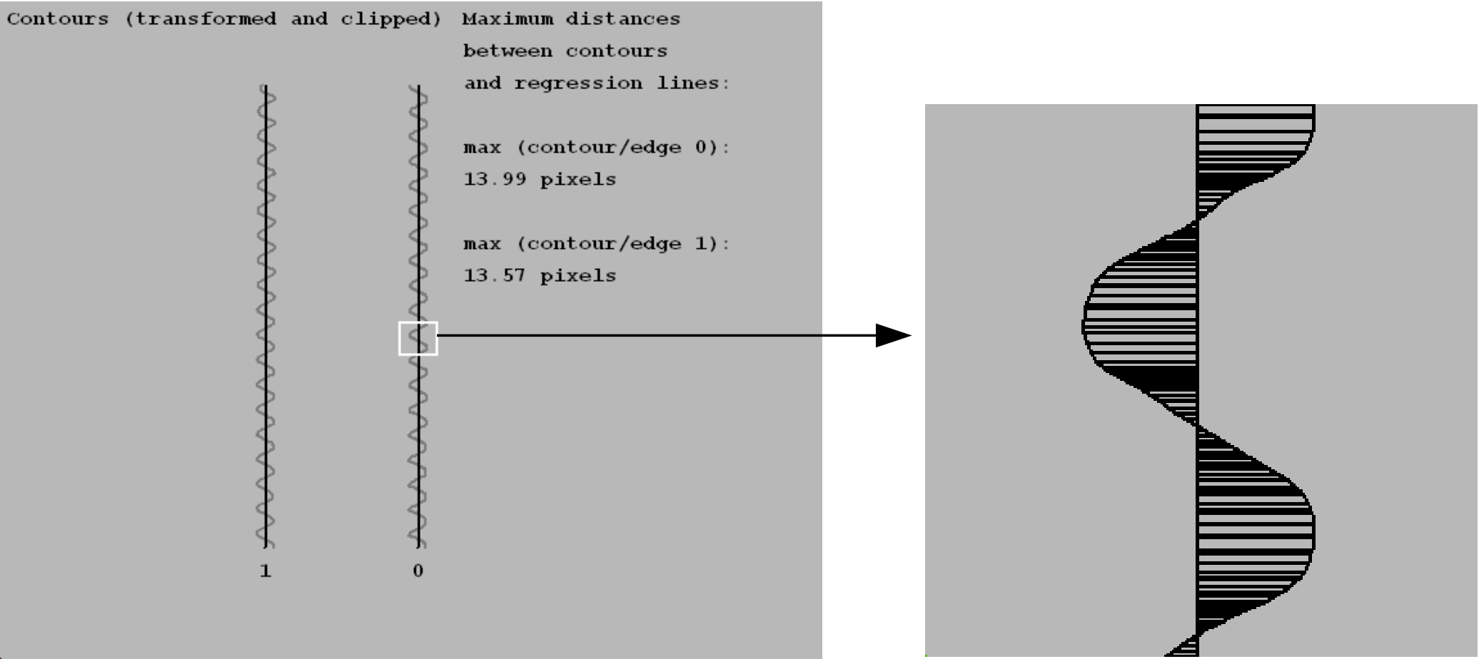
Steps within the example:
-
Create ROI.
Region processing is used to create an ROI for the following contour processing. For this, we reduce the original region of the screw to its border by the operatorboundary (Region, RegionBorder, 'inner_filled') dilation_circle (RegionBorder, RegionDilation, 7.5) reduce_domain (Image, RegionDilation, ImageReduced)boundaryand use the morphological operatordilation_circleto enlarge it. The domain is reduced to the enlarged region byreduce_domain. -
Extract and transform contours.
The ROI is used as search space for the contour processing that starts with a subpixel-precise edge extraction. Because we need the outer parts of the contour, a curve flattening must be avoided. Thus, we use a Laplace filter, which leads to less smooth edges but matches the turning parts of the contour. It is applied using the operatorsigma := 3 derivate_gauss (ImageReduced, DerivGauss, sigma, 'laplace') zero_crossing_sub_pix (DerivGauss, Edges) select_contours_xld (Edges, SelectedEdges, 'contour_length', 3000, 99999, \ -0.5, 0.5)derivate_gausswith the parameter laplace.The
zero_crossing_sub_pixthen returns the edge contours. From these, we select the contours with a minimum size usingselect_contours_xld. The operatoraffine_trans_contour_xldthen transforms the contours using the same homogeneous transformation matrix as used for the transformation of the region obtained beforehand.
Withaffine_trans_contour_xld (SelectedEdges, ContoursAffineTrans, \ HomMat2DRotate)smallest_rectangle1_xldandclip_contours_xld, the now vertical contour is clipped to get that part of the screw’s border that contains the two separated thread edges on the left and right side of the screw.smallest_rectangle1_xld (ContoursAffineTrans, Row11, Column11, Row21, \ Column21) clip_contours_xld (ContoursAffineTrans, ClippedContours, Row11 + 90, 0, \ Row21 - 90, Width)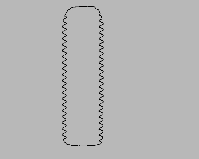
Figure 4: Extracted and transformed contours of the screw -
Get regression lines.
The operatorfit_line_contour_xld (ClippedContours, 'regression', -1, 0, 5, 2, RowBegin, \ ColBegin, RowEnd, ColEnd, Nr, Nc, Dist1)fit_line_contour_xldnow uses the contours to compute the start (RowBegin,ColBegin) and end (RowEnd,ColEnd) points for the regression lines.To get the points of the regression lines, the parameter Algorithm must be set to
regression. Until now, we handled both contours together in tuples.The tuple
Edgescontains the contours of the two thread edges, and the tuples for the start and end points of the regression lines contain the points for both regression lines.With the operator
gen_contour_polygon_xldwe explicitly create the contours of the individual regression lines. For this, we use the corresponding start and end points as input.For the first regression line
RegressContour0we use the start and end points with the index0, and for the second regression lineRegressContour1we use the elements with index1.gen_contour_polygon_xld (RegressContour0, [RowBegin[0],RowEnd[0]], \ [ColBegin[0],ColEnd[0]]) gen_contour_polygon_xld (RegressContour1, [RowBegin[1],RowEnd[1]], \ [ColBegin[1],ColEnd[1]])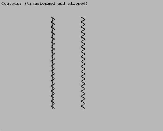
Figure 5: Clipped contours and the corresponding regression lines -
Extract contour points of the thread edges.
To get the deviation between the thread contours and their corresponding regression lines, we additionally need the contour points of the thread contours. The thread contours are stored both in the tupleselect_obj (ClippedContours, EdgeContour0, 1) get_contour_xld (EdgeContour0, RowEdge0, ColEdge0) select_obj (ClippedContours, EdgeContour1, 2) get_contour_xld (EdgeContour1, RowEdge1, ColEdge1)Edges. Since we want to access the individual contours more than once, the usage of the indices may become a little bit confusing.To make the code clearer and also to apply further tuple operations to each contour later on, we select the elements of the tuple individually and assign concise names to them, for example
EdgeContour0andEdgeContour1.The selection of iconic objects is not realized via an assign statement but by the operator
select_obj. Note that the index of iconic objects starts with 1 instead of 0. For the thread contoursEdgeContour0andEdgeContour1, a tuple containing the rows and columns of the contour points is obtained withget_contour_xld. -
Calculate the horizontal distances.
The obtained contour points are used to calculate the distances between each contour point of the thread edge and the contour of the corresponding regression line.distance_pc (RegressContour0, RowEdge0, ColEdge0, DistanceMin0, \ DistanceMax0) minDistance0 := min(DistanceMin0) maxDistance0 := max(DistanceMin0) meanDistance0 := mean(DistanceMin0)The operator
distance_pcreturns the minimum and maximum distances. The minimum distances between the contour points and the contour of the regression line correspond to the horizontal distances in approximately each row, as long as the screw is vertical. These in turn can be used to query the minimum, maximum, and mean horizontal distance between both contours.The code only shows the proceeding for
EdgeContour0andRegressContour0. -
Visualize the result in a zoom window.
To visualize the individual horizontal distances between a thread contour and its regression line in a zoom window, the endpoints of the regression line are made explicit by the contour points and with these, the points of the thread contour are projected onto the regression line usingdev_display (EdgeContour0) dev_display (RegressContour0) get_contour_xld (RegressContour0, RowContour0, ColContour0) for i := 800 to 950 by 1 projection_pl (RowEdge0[i], ColEdge0[i], RowContour0[0], ColContour0[0], \ RowContour0[1], ColContour0[1], RowProj0, ColProj0) gen_contour_polygon_xld (Contour, [RowEdge0[i],RowProj0], [ColEdge0[i], \ ColProj0]) dev_display (Contour) endforprojection_pl.The lines between the points and their projections are created by
gen_contour_polygon_xldand visualized by the standard visualization operatordev_display.
Getting the distance between straight parallel contours🔗
Using contours obtained by line fitting🔗
A third measuring approach realized in the example program %HALCONEXAMPLES%\solution_guide\ 2d_measuring\measure_screw measures the distance between the two parallel contours of the regression lines RegressContour0 and RegressContour1, which were obtained beforehand.
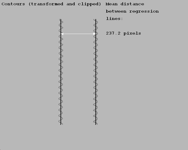
For this, we compute the distances between the end points of the regression lines using the operator distance_pp.
distance_pp (RowBegin[1], ColBegin[1], RowEnd[0], ColEnd[0], Distance1)
distance_pp (RowBegin[0], ColBegin[0], RowEnd[1], ColEnd[1], Distance2)
if (abs(Distance1 - Distance2) < 1)
    disp_message (WindowID, 'Mean distance', 'image', 10, 720, 'black', \
                  'false')
    disp_message (WindowID, 'between regression', 'image', 60, 720, 'black', \
                  'false')
    disp_message (WindowID, 'lines:', 'image', 110, 720, 'black', 'false')
    disp_message (WindowID, ((Distance1 + Distance2) / 2)$'.4' + ' pixels', \
                  'image', 210, 720, 'black', 'false')
endif
Before displaying the mean width of the object, we check if the distance between the two points at the top of the screw correspond to the distance between the points at the bottom, that is, we check if the lines are parallel within a certain tolerance.
Using polygons instead of lines🔗
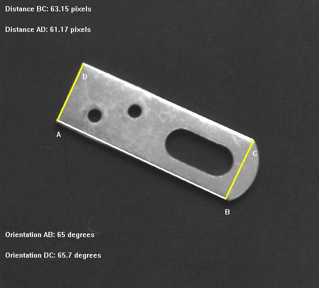
The example program %HALCONEXAMPLES%\solution_guide\2d_measuring\ measure_metal_part_extended demonstrates a similar approach.
As before, a contour is extracted and segmented into linear and circular contour segments, the segments are stored in the tuple ContoursSplit.
gen_polygons_xld (ContoursSplit, Polygons, 'ramer', 2)
gen_parallels_xld (Polygons, Parallels, 80, 75, 0.15, 'true')
count_obj (Parallels, NumberParallels)
for i := 1 to NumberParallels by 1
    select_obj (Parallels, SelectedParallel, i)
    get_parallels_xld (SelectedParallel, Row1Parallels, Col1Parallels, \
                       Length1Parallels, Phi1Parallels, Row2Parallels, \
    Col2Parallels, Length2Parallels, Phi2Parallels)
    distance_pp (Row1Parallels[0], Col1Parallels[0], Row2Parallels[1], \
                 Col2Parallels[1], Distance2)
    distance_pp (Row1Parallels[1], Col1Parallels[1], Row2Parallels[0], \
                 Col2Parallels[0], Distance1)
endfor
In contrast to the approach described before, instead of fitting lines, the linear segments are approximated by olygons using gen_polygons_xld.
From these polygons, the approximately parallel lines Parallels can be explicitly extracted by gen_parallels_xld.
To get the end points and orientation of the corresponding line segments, we apply the operator get_parallels_xld for each pair of parallel lines.
The number of pairs, needed for creating the for loop, is obtained by the operator count_obj, which counts the number of objects of a tuple containing iconic data.
For control data, an assign statement would be used.
For a pair of parallel lines we now calculate the distances between the opposed end points with the geometric operation distance_pp.
Using the smallest enclosing rectangle🔗
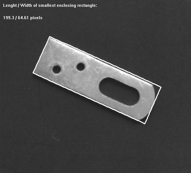
A complex shape that is delimited by straight lines that are known to be parallel and you want to know the distance between them, you can also obtain the width of the object by computing the smallest enclosing rectangle for it.
To do so, you do not even have to extract the individual segments, but extract the region or contour of the object and then apply smallest_rectangle2 to the region or smallest_rectangle2 to the contour.
Depending on the dimension of your object, the returned parameter Length1 or Length2 then represents half of the distance between the parallel lines.
For contours that approximate a rectangle, the fitting of rectangles to contours using fit_rectangle2_contour_xld is suitable.
Getting the width of linear structures🔗
To get the width of thin linear structures, the operator lines_gauss can be used.
Note
The linear structures are called lines, but in contrast to the XLD lines obtained by a line fitting, they are built by edge pairs, and for each line attributes like the width can be stored and queried.
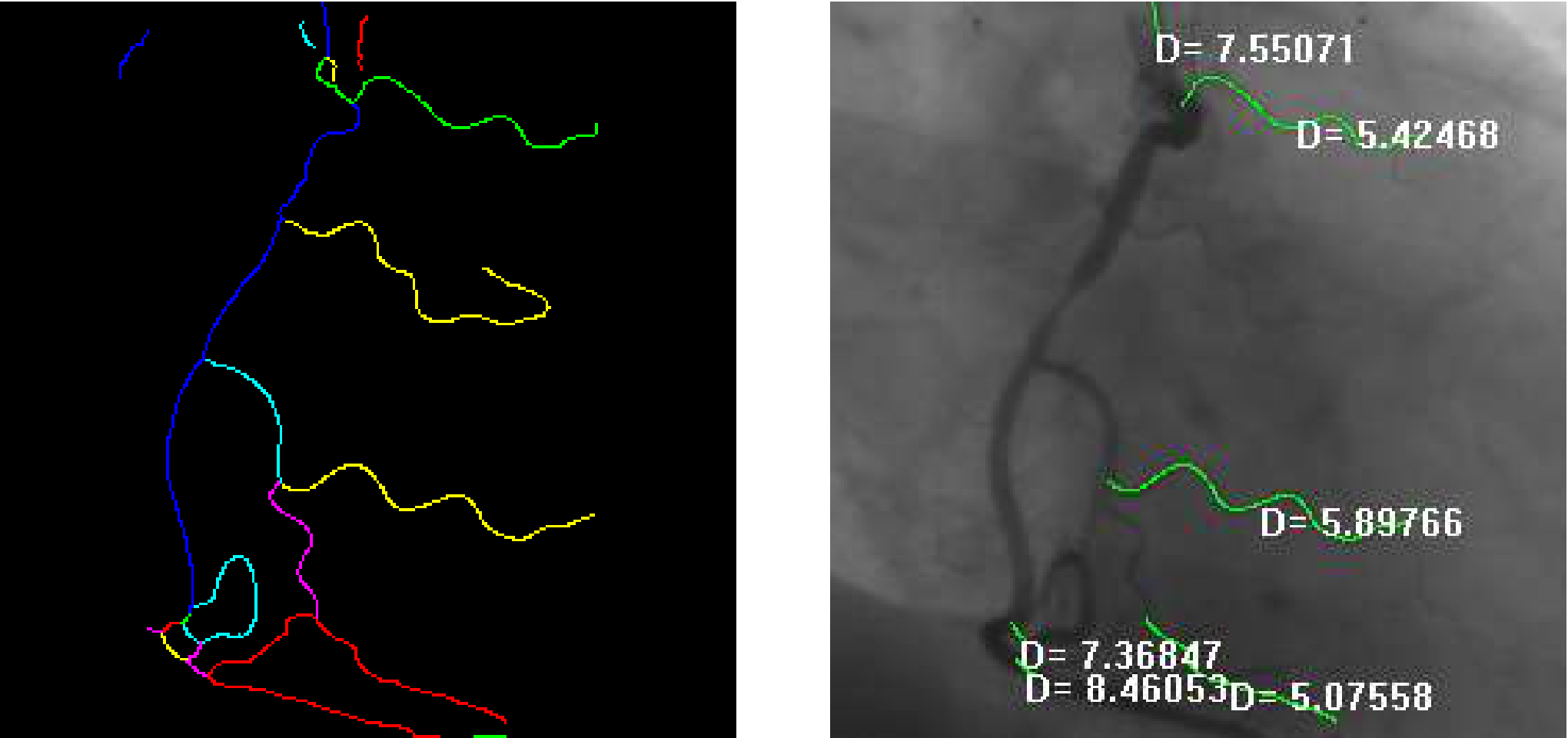
lines_gauss in the example angio: extracted lines (left), visualization of the diameters of the selected lines (right) Examples showing how to apply the operator are:
%HALCONEXAMPLES%\hdevelop\Applications\Measuring-2D\angio%HALCONEXAMPLES%\hdevelop\Filters\Lines\lines_gauss
You can select whether bright or dark lines are detected and adjust parameters for the general line extraction.
Parameters can be set that control which attributes are stored with the obtained lines.
These attributes can then be queried with the operator get_contour_attrib_xld.
Depending on the selected parameters in lines_gauss you can query the following parameters:
- The angle of the direction perpendicular to the line
angle. - The magnitude of the second derivative
response. - The line widths to the left or to the right of the line
width_left,width_right. - The asymmetry of a line point
asymmetry. - The contrast of a line point
contrast.
Getting lines and junctions of a grid🔗
The example program %HALCONEXAMPLES%\solution_guide\2d_measuring\measure_grid inspects a numeric keypad. In particular, the positions of the junctions of the grid separating the keys are measured.
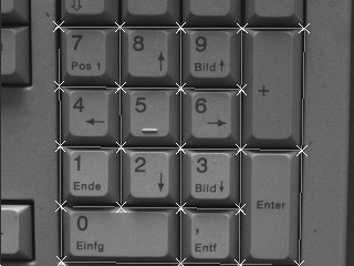
Steps within the example:
-
Get region between and around the keys.
The region representing the space between and around the keys is segmented and further processed via region processing. This includes the coarse segmentation of the image via a dynamic threshold (mean_image (Image, ImageMean, 7, 7) dyn_threshold (Image, ImageMean, RegionDynThresh, 4, 'dark') connection (RegionDynThresh, ConnectedRegions) select_shape (ConnectedRegions, SelectedRegions, ['max_diameter', \ 'contlength'], 'and', [200, 800], [99999, 99999]) closing_circle (SelectedRegions, RegionClosing, 1.5)dyn_threshold), the selection of a connected region of a certain size (connectionfollowed byselect_shape), as well as the closing of small gaps byclosing_circle. -
Get skeleton and the corresponding horizontal and vertical linear contours.
The region is reduced to itsskeleton (RegionClosing, Skeleton) gen_contours_skeleton_xld (Skeleton, ContoursSkeleton, 1, 'filter') segment_contours_xld (ContoursSkeleton, ContoursSplitSkeleton, 'lines', 5, \ 2, 1) select_contours_xld (ContoursSplitSkeleton, SelectedContours, \ 'contour_length', 30, 1000, -0.5, 0.5) union_collinear_contours_xld (SelectedContours, UnionCollinearContours, 100, \ 10, 20, rad(10), 'attr_keep')skeleton, which is then transformed to a contour bygen_contours_skeleton_xld. The contour is segmented into individual lines (segment_contours_xld), from which those are selected byselect_contours_xldthat have a minimum contour length.Additionally, collinear lines are merged by
union_collinear_contours_xld.The lines are fitted to each contour by
fit_line_contour_xldand the corresponding line contours are generated bygen_contour_polygon_xld.For each contour, the orientation is checked within a tolerance of 0.05 rad in both directions and horizontal lines are stored in the tuple
LinesHorizontaland vertical lines in the tupleLinesVertical. Both are first created bygen_empty_objand then successively filled usingconcat_obj.count_obj (UnionCollinearContours, NumberContours) gen_empty_obj (LinesHorizontal) gen_empty_obj (LinesVertical) for i := 1 to NumberContours by 1 select_obj (UnionCollinearContours, ObjectSelected, i) fit_line_contour_xld (ObjectSelected, 'tukey', -1, 0, 5, 2, RowBegin, \ ColBegin, RowEnd, ColEnd, Nr, Nc, Dist) gen_contour_polygon_xld (Contour, [RowBegin,RowEnd], [ColBegin,ColEnd]) Phi := atan2(-Nr,Nc) if (abs(Phi) < rad(5)) concat_obj (LinesVertical, Contour, LinesVertical) endif if (rad(85) < abs(Phi) and abs(Phi) < rad(95)) concat_obj (LinesHorizontal, Contour, LinesHorizontal) endif endfor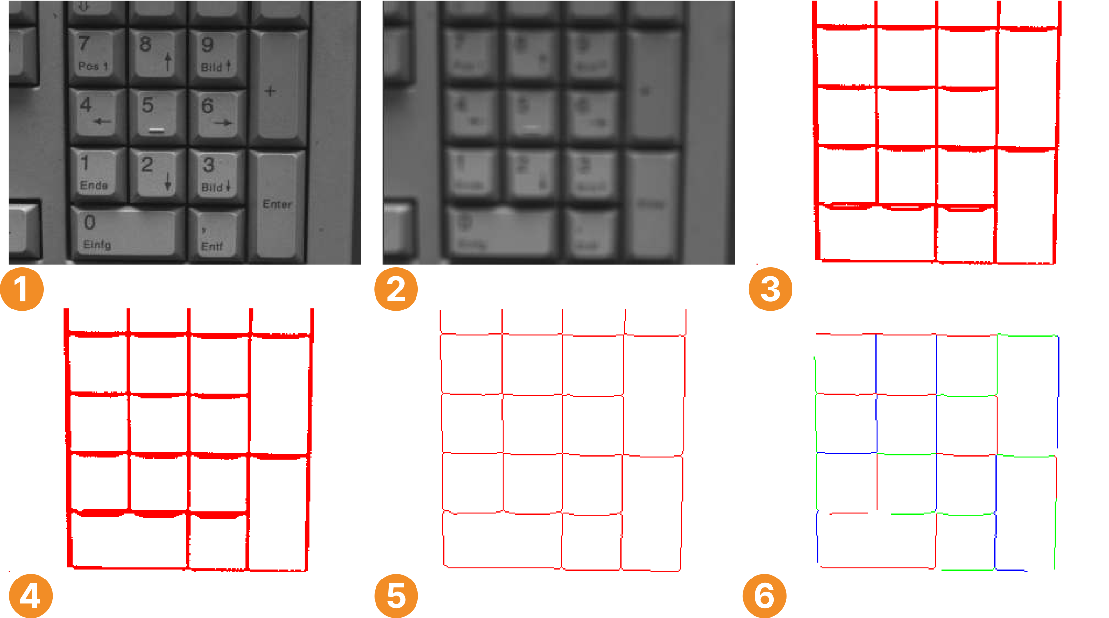
Original image
Image processed
Extracted region with gaps
Region after closing gaps by a morphological operator
Skeleton
Selected contour segments
-
Get junction points.
Inside a loop, each horizontal line is intersectedRowJunction := [] ColJunction := [] RowRealJunction := [] ColRealJunction := [] count_obj (LinesHorizontal, NumberLH) count_obj (LinesVertical, NumberLV) for i := 1 to NumberLH by 1 select_obj (LinesHorizontal, HorizontalLine, i) get_contour_xld (HorizontalLine, RowHorizontal, ColHorizontal) for j := 1 to NumberLV by 1 select_obj (LinesVertical, VerticalLine, j) get_contour_xld (VerticalLine, RowVertical, ColVertical) intersection_lines (RowHorizontal[0], ColHorizontal[0], \ RowHorizontal[1], ColHorizontal[1], \ RowVertical[0], ColVertical[0], RowVertical[1], \ ColVertical[1], Row, Column, IsOverlapping) distance_ps (Row, Column, RowHorizontal[0], ColHorizontal[0], \ RowHorizontal[1], ColHorizontal[1], DistanceH, \ DistanceHMax) distance_ps (Row, Column, RowVertical[0], ColVertical[0], \ RowVertical[1], ColVertical[1], DistanceV, \ DistanceVMax) RowJunction := [RowJunction,Row] ColJunction := [ColJunction,Column]intersection_lineswith each vertical line to get the junction points of the regular grid. This grid is built by lines of infinite length, so that the intersection leads to junction points also at the large keys. -
Reduce the point set.
To get only those points of the grid that represent a real existing junction, for each junction point the distances to the two line segments used for its creation are computed byif ((DistanceH <= 30) and (DistanceV <= 30)) RowRealJunction := [RowRealJunction,Row] ColRealJunction := [ColRealJunction,Column] endif endfor endfordistance_ps. If both distances are less than 30 pixels, the point is assumed to be a real junction point. -
Obtain junction points via region processing.
Junction points can also be obtained via region processing. Here, we apply
junctions_skeletonto the skeleton we obtained before. Since the operator returns regions instead of points, we applyget_region_pointsto get the center positions of each junction.junctions_skeleton (Skeleton, EndPoints, JuncPoints) get_region_points (JuncPoints, RowJunctionRegionProcessing, \ ColumnJunctionRegionProcessing) gen_cross_contour_xld (CrossCenter, RowJunctionRegionProcessing, \ ColumnJunctionRegionProcessing, 12, 0.785398)In contrast to contour processing these junction positions are not based on a grid obtained by straight lines but on the region extracted between the keys. Depending on the region, the resulting junction points may be ambiguous and may not represent junctions of a regular grid.
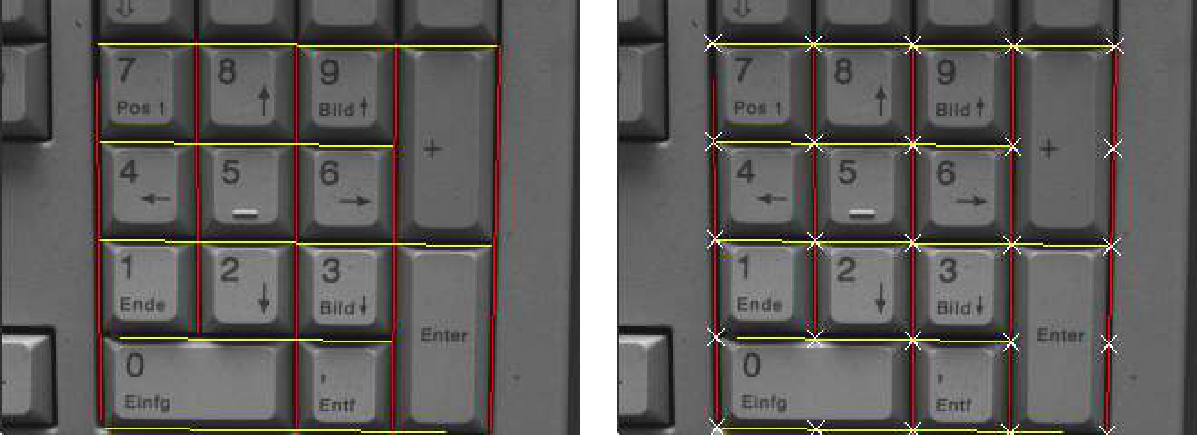
Figure 11: Collinear horizontal and vertical contours obtained by line fitting (left), all junctions of the regular grid including junctions that do not represent a real existing junction between keys (right)
Getting positions of corner points🔗
The example program %HALCONEXAMPLES%\solution_guide\ 2d_measuring\measure_metal_part_extended extracts the positions of the corners of a metal plate in an image by two different approaches.
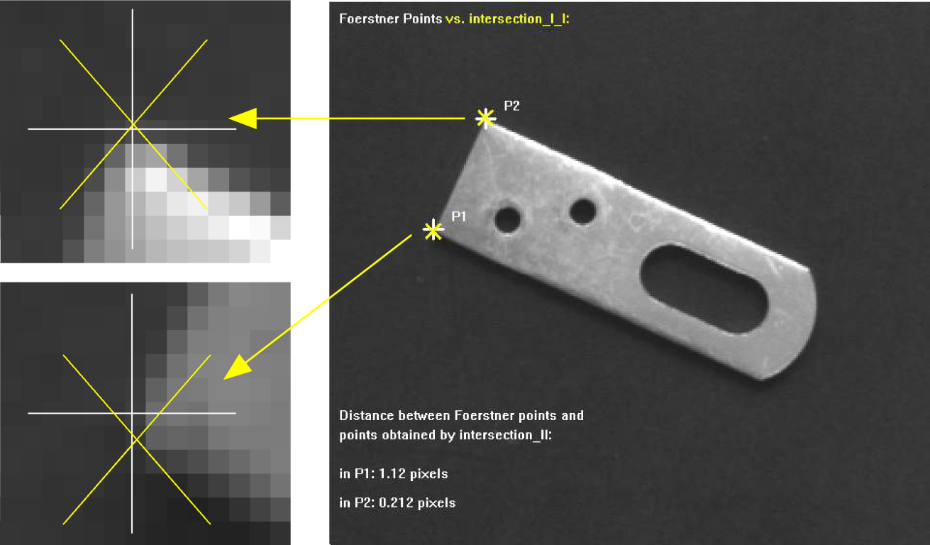
Steps within the example:
-
Get Förstner points.
The first approach is realized by a point operator. Here, the points, row and column coordinates stored in the tuplespoints_foerstner (Image, 1, 2, 3, 200, 0.3, 'gauss', 'false', RowJunctions, \ ColJunctions, CoRRJunctions, CoRCJunctions, \ CoCCJunctions, RowArea, ColArea, CoRRArea, CoRCArea, \ CoCCArea)RowJunctionsandColJunctions, are extracted bypoints_foerstner. -
Get corner points by line intersection.
The second approach intersects lines to get the positions of the corners. The adjacent lines building the corners are obtained by line fitting, so that edges are extracted usingedges_sub_pix (ImageReduced, Edges, 'lanser2', 0.5, 40, 90) segment_contours_xld (Edges, ContoursSplit, 'lines_circles', 6, 4, 4) sort_contours_xld (ContoursSplit, SortedContours, 'upper_left', 'true', \ 'column') count_obj (SortedContours, NumSegments) for i := 1 to NumSegments by 1 select_obj (SortedContours, SingleSegment, i) get_contour_global_attrib_xld (SingleSegment, 'cont_approx', Attrib) fit_line_contour_xld (SingleSegment, 'tukey', -1, 0, 5, 2, RowBegin, \ ColBegin, RowEnd, ColEnd, Nr, Nc, Dist) RowsBegin := [RowsBegin,RowBegin] ColsBegin := [ColsBegin,ColBegin] RowsEnd := [RowsEnd,RowEnd] ColsEnd := [ColsEnd,ColEnd] endforedges_sub_pix, the obtained contours are segmented bysegment_contours_xldand sorted bysort_contours_xld, and to each linear segment a line is fitted viafit_line_contour_xld.The returned end points of the lines are stored in the tuples
RowsBegin,ColsBegin,RowsEnd, andColsEnd.From these end points, the intersection points of the lines (
RowIntersect*,ColIntersect*) are calculated viaintersection_lines.intersection_lines (RowsBegin[0], ColsBegin[0], RowsEnd[0], ColsEnd[0], \ RowsBegin[1], ColsBegin[1], RowsEnd[1], ColsEnd[1], \ RowIntersect1, ColumnIntersect1, IsOverlapping1) intersection_lines (RowsBegin[0], ColsBegin[0], RowsEnd[0], ColsEnd[0], \ RowsBegin[2], ColsBegin[2], RowsEnd[2], ColsEnd[2], \ RowIntersect2, ColumnIntersect2, IsOverlapping2) -
Compare the two approaches.
To compare the results of both approaches, the distances between the points obtained by the line intersection and their corresponding Förstner points are computed bydistance_pp (RowJunctions[1], ColJunctions[1], RowIntersect1, \ ColumnIntersect1, Distance1) distance_pp (RowJunctions[0], ColJunctions[0], RowIntersect2, \ ColumnIntersect2, Distance2)distance_pp.
Getting the angle between adjacent lines🔗
With the end points of the adjacent lines obtained beforehand, we now can use the geometric operation angle_ll to get the angle between the adjacent lines and check whether both angles are exactly or only approximately right angled.
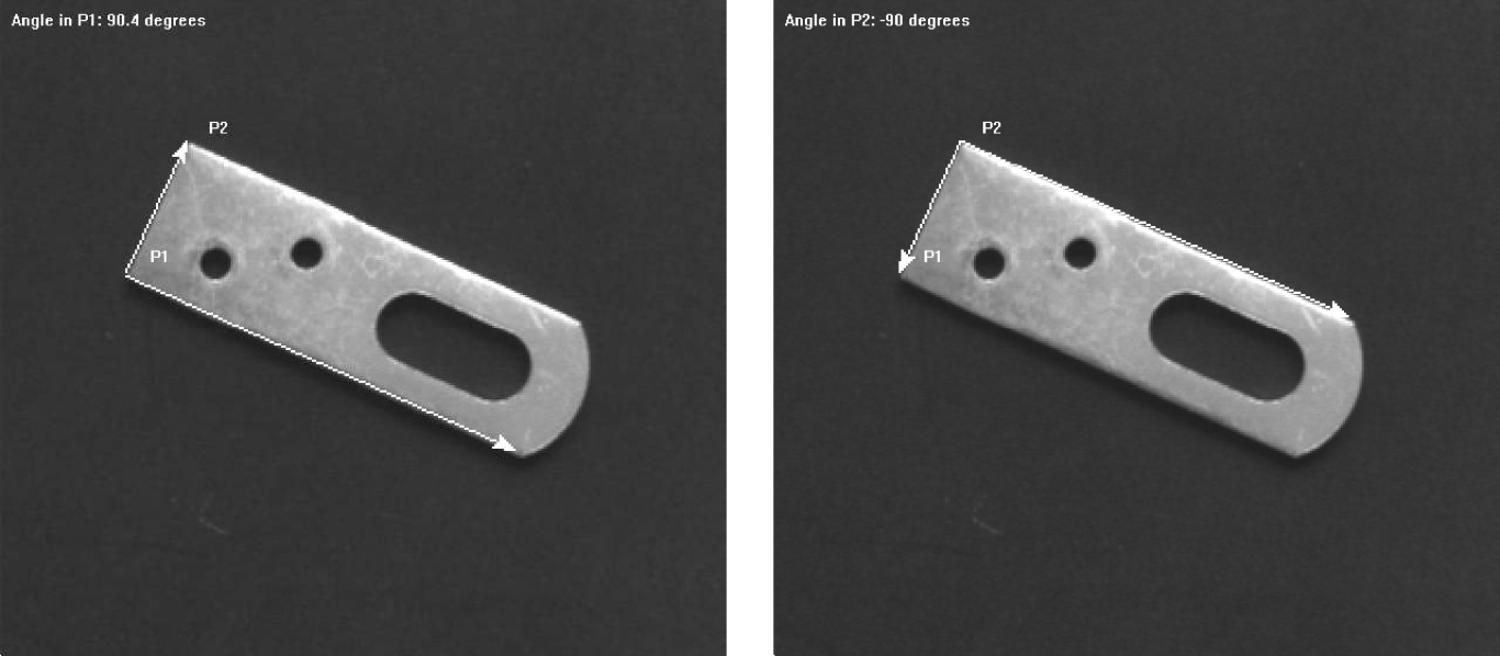
angle_ll (RowsBegin[0], ColsBegin[0], RowsEnd[0], ColsEnd[0], RowsBegin[1], \
          ColsBegin[1], RowsEnd[1], ColsEnd[1], Angle1)
angle_ll (RowsBegin[0], ColsBegin[0], RowsEnd[0], ColsEnd[0], RowsBegin[2], \
          ColsBegin[2], RowsEnd[2], ColsEnd[2], Angle2)
Getting positions, orientations, and extents of rectangles🔗
The example program %HALCONEXAMPLES%\solution_guide\2d_measuring\measure_chip extracts the rectangular shapes of the die and the frame of a chip.
The relations between the two positions and orientations are needed, for example for a correct die bonding.
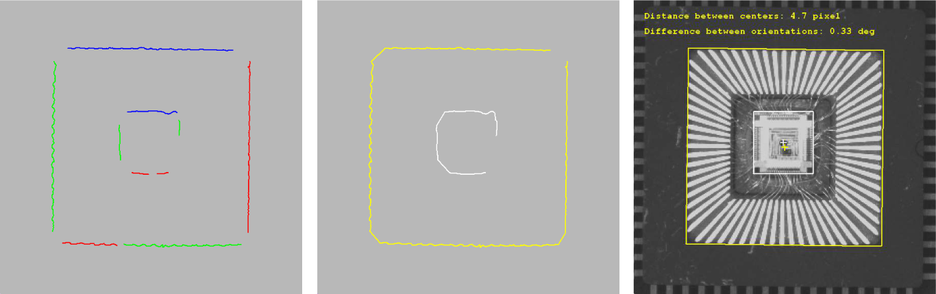
Steps within the example:
-
Create ROI for the die.
The program starts with region processing. It coarsely determines the region of the die usingfast_threshold (Image, Region, 120, 255, 20) opening_rectangle1 (Region, RegionOpening, 4, 4) connection (RegionOpening, ConnectedRegions) fill_up (ConnectedRegions, RegionFillUp) select_shape (RegionFillUp, SelectedRegions, ['rectangularity', 'area'], \ 'and', [0.8, 700], [1, 99999]) smallest_rectangle2 (SelectedRegions, Row, Column, Phi, Length1, Length2) gen_rectangle2 (Rectangle, Row, Column, Phi, Length1, Length2)fast_threshold. The operatoropening_rectangle1suppresses the small wires.After separating the individual connected parts of the region with connection, we
fill_upthe remaining holes and select a region of rectangular shape and a certain sizeselect_shape.The region is approximated by its smallest enclosing rectangle
smallest_rectangle2andgen_rectangle2, which lead to a pixel-precise approximation for the position, orientation, and extent of the rectangle.Because we need subpixel precision here, region processing is not sufficient. The region of the rectangle is reduced to its slightly enlarged boundary (
boundaryfollowed bydilation_rectangle1) and the reduced image (obtained byreduce_domain) is used as ROI, it builds the search space for the following contour processing.boundary (Rectangle, RegionBorder, 'inner_filled') dilation_rectangle1 (RegionBorder, RegionDilation, 4, 4) reduce_domain (Image, RegionDilation, ImageReduced) -
Extract contours of the die.
Inside the ROI, the subpixel-precise edges of the die’s border are extracted by the operatoredges_sub_pix (ImageReduced, Edges, 'canny', 1.5, 30, 40) segment_contours_xld (Edges, ContoursSplit, 'lines', 5, 2, 2) select_contours_xld (ContoursSplit, SelectedContours1, 'contour_length', 10, \ 99999, -0.5, 0.5) union_adjacent_contours_xld (SelectedContours1, UnionContours1, 30, 1, \ 'attr_keep')edges_sub_pix.The edges are segmented into linear contours using the operator
segment_contours_xldwith the parameterModeset tolines.The contours having a minimum length are selected by
select_contours_xld. The contours that belong to the border are now adjacent within a certain tolerance.To merge the contours that are neighboring within a range of 30 pixels, the operator
union_adjacent_contours_xldis applied. -
Fit rectangle to the contours of the die.
The operatorfit_rectangle2_contour_xld (UnionContours1, 'tukey', -1, 0, 0, 3, 2, Row1, \ Column1, Phi1, Length11, Length12, PointOrder1) gen_rectangle2_contour_xld (Rectangle1, Row1, Column1, Phi1, Length11, \ Length12)fit_rectangle2_contour_xlduses the obtained contour to get the position, orientation, and extent of the best-fitting rectangle of the die. The corresponding rectangle is then created bygen_rectangle2_contour_xld. -
Create ROI and extract contours of the frame.
A similar procedure is applied for the border of the frame. The extraction of the ROI is slightly different because the appearance of both objects in the image differs.threshold_sub_pix (ImageReduced1, Border1, 70)The operator
threshold_sub_pixextracts the contours. The ROI in this case is needed to reduce the number of contours to investigate rather than to reduce the runtime of the contour extraction.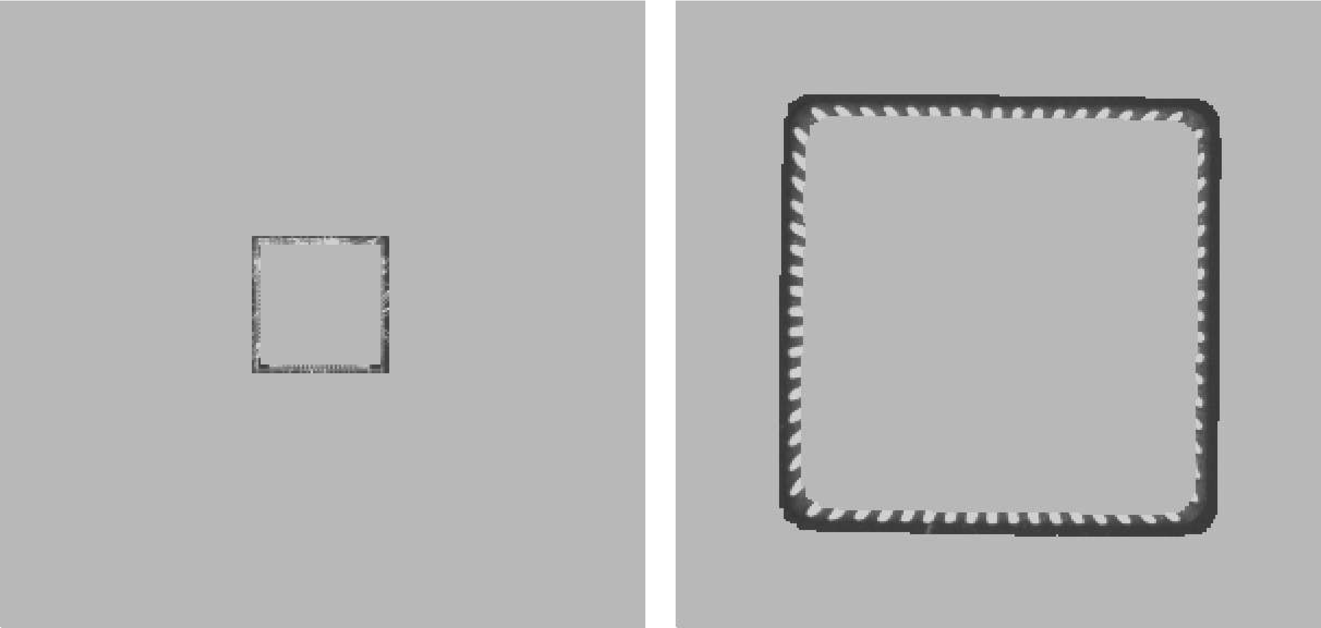
Figure 15: ROIs for the rectangle fitting: ROI for the die (left), ROI for the frame (right) -
Fit rectangle to the contours of the frame.
Again, the adjacent contours are merged, the parameters of the best-fitting rectangle are obtained for the merged contour, and the corresponding rectangle is created and displayed.
-
Compare the position and orientation of both rectangles.
With the parameters of the rectangles for both shapes, the distance between their center positions (distance_pp (Row1, Column1, Row2, Column2, Distance)distance_pp) and the difference between their orientations are calculated.Phi1andPhi2were obtained automatically by the rectangle fitting.
Getting radii of circles and circular arcs🔗
The example program %HALCONEXAMPLES%\solution_guide\2d_measuring\measure_circles extracts the radii of circular shapes that are punched out of a metal plate.
The image of the plate is acquired using a back light to get a good contrast between fore- and background.
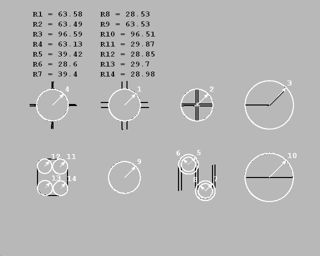
Steps within the example:
-
Create ROI.
To extract the bright regions of the circular shapes afast_threshold (Image, Region, 200, 255, 20) connection (Region, ConnectedRegions) select_shape (ConnectedRegions, SelectedRegions, 'area', 'and', 70, 50000) boundary (SelectedRegions, RegionBorder, 'inner_filled') dilation_circle (RegionBorder, RegionDilation, 3.5) union1 (RegionDilation, RegionUnion) reduce_domain (Image, RegionUnion, ImageReduced)fast_thresholdis applied. Connected regions are separated by connection and regions with a minimum size are selected for the further processing usingselect_shape.The regions are restricted to their borders by the operator
boundary. These borders are enlarged a bit by a dilationdilation_circle.The dilated regions are merged by the operator
union1so that the image can be reduced to a region that contains all parts needed for the further tasks usingreduce_domain.The reduced image is used as an ROI, it builds the search space for the subpixel-precise edge extraction.
-
Extract circular contour segments.
The edges obtained byedges_sub_pix (ImageReduced, Edges, 'canny', 1.5, 10, 40) segment_contours_xld (Edges, ContoursSplit, 'lines_circles', 5, 2, 2) select_contours_xld (ContoursSplit, SelectedContours, 'contour_length', 25, \ 99999, -0.5, 0.5) count_obj (SelectedContours, NumberContours) gen_empty_obj (Circles) for i := 1 to NumberContours by 1 select_obj (SelectedContours, ObjectSelected, i) get_contour_global_attrib_xld (ObjectSelected, 'cont_approx', Attrib) if (Attrib == 1) concat_obj (Circles, ObjectSelected, Circles) endif endfor union_cocircular_contours_xld (Circles, UnionContours, rad(60), rad(10), \ rad(30), 100, 50, 10, 'true', 1)edges_sub_pixare segmented into linear and circular segments bysegment_contours_xld.Because more contours exist than needed for the circle extraction, only the contours having a minimum contour length are selected by
select_contours_xld.For these, it is checked if they are circular, the value for
cont_approxis queried byget_contour_global_attrib_xldand if it is1, the contour is stored in the tupleCircles.All circular contours that lie approximately on the same circle are merged by
union_cocircular_contours_xld. These contours are now used for the circle fitting.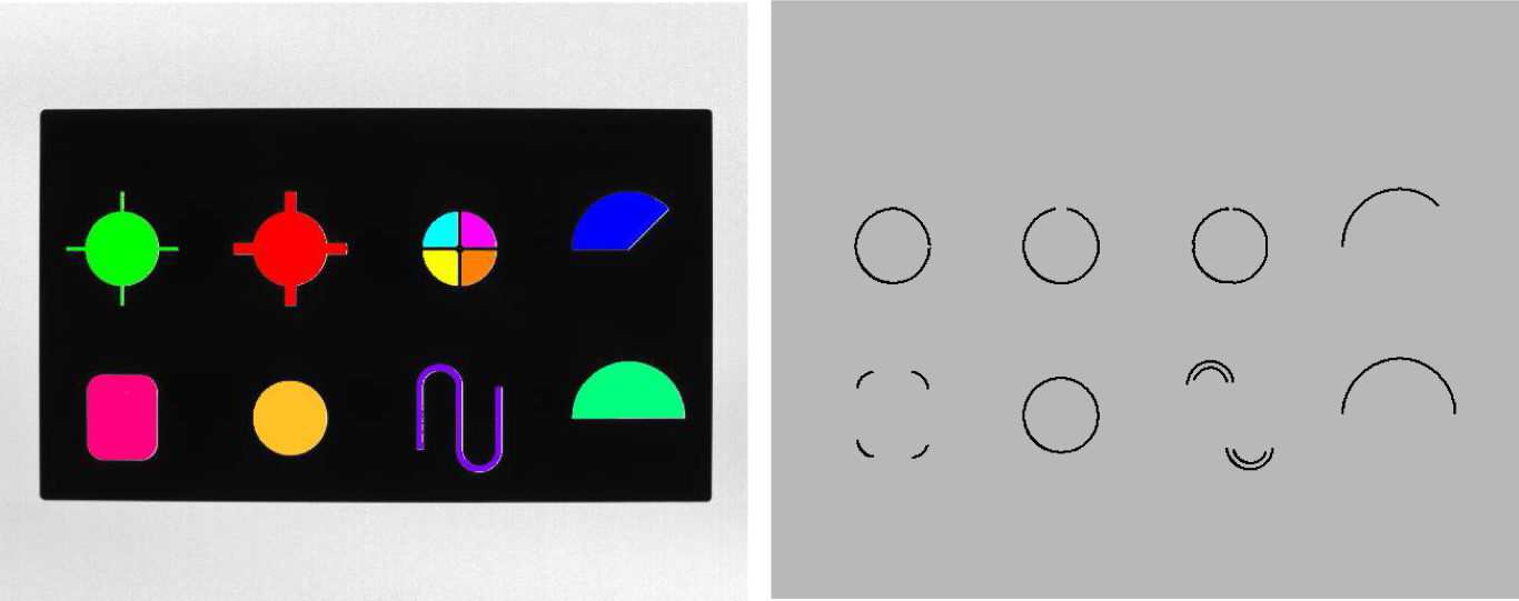
Figure 17: Circle fitting: Original image overlaid by the extracted regions (left), circular contours selected for the circle fitting (right) -
Fit circles to the circular contour segments.
For the circle fitting, the operatorcount_obj (UnionContours, NumberCircles) for i := 1 to NumberCircles by 1 select_obj (UnionContours, ObjectSelected, i) fit_circle_contour_xld (ObjectSelected, 'algebraic', -1, 0, 0, 3, 2, \ Row, Column, Radius, StartPhi, EndPhi, \ PointOrder) gen_circle_contour_xld (ContCircle, Row, Column, Radius, 0, rad(360), \ 'positive', 1.5) dev_display (ContCircle) endforfit_circle_contour_xldis applied to each contour. It returns, amongst others, the center and radius of the circle that fits best to the contour. The corresponding circle is generated with the operatorgen_circle_contour_xld, which then can be displayed or processed further.
Getting the deviation of a contour from a circle🔗
The example program %HALCONEXAMPLES%\solution_guide\2d_measuring\measure_pump shows a second example for the extraction of circles in an image.
Here, not only the radius of a best-fitting circle must be found for a contour, but also the deviation of the contour from the circle.
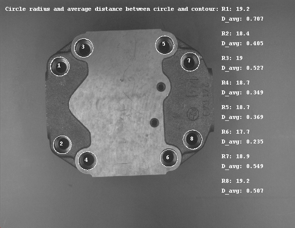
Steps within the example:
-
Create ROI.
The approach, like others before, starts with the creation of a suitable ROI.fast_threshold (Image, Region, 0, 70, 150) connection (Region, ConnectedRegions) select_shape (ConnectedRegions, SelectedRegions, ['outer_radius', \ 'anisometry', 'area'], 'and', [5, 1, 100], [50, 1.8, 99999]) shape_trans (SelectedRegions, RegionTrans, 'outer_circle') dilation_circle (RegionTrans, RegionDilation, 5.5) union1 (RegionDilation, RegionUnion) reduce_domain (Image, RegionUnion, ImageReduced)fast_thresholdis applied, the connected regions are separated byconnection, shapes with a certain outer radius, anisometry, and area are selected usingselect_shape, and the regions are transformed into their outer circles byshape_trans.These circles are enlarged by
dilation_circle, the regions are merged into a single region byunion1, and the image is reduced to the obtained regionreduce_domain.The reduced image builds the search space for the contour processing.
-
Extract circular contour segments.
Contours are created using the operatorthreshold_sub_pix (ImageReduced, Border, 80) select_shape_xld (Border, SelectedXLD, ['contlength', 'outer_radius'], \ 'and', [70, 15], [99999, 99999]) segment_contours_xld (SelectedXLD, ContoursSplit, 'lines_circles', 4, 2, 2) select_shape_xld (ContoursSplit, SelectedXLD3, ['outer_radius', \ 'contlength'], 'and', [15, 30], [45, 99999]) union_cocircular_contours_xld (SelectedXLD3, UnionContours2, 0.5, 0.1, 0.2, \ 2, 10, 10, 'true', 1) sort_contours_xld (UnionContours2, SortedContours, 'upper_left', 'true', \ 'column')threshold_sub_pix. To select the relevant contours from the obtained set of contours, the operatorselect_shape_xldis applied, searching for contours of a specific length and with a certain outer radius. The relevant contours are then segmented into lines and circles withsegment_contours_xld. From the segments, again contours with a specific contour length and outer radius are selected. Cocircular contours are merged byunion_cocircular_contours_xld, and finally the contours are sorted bysort_contours_xld.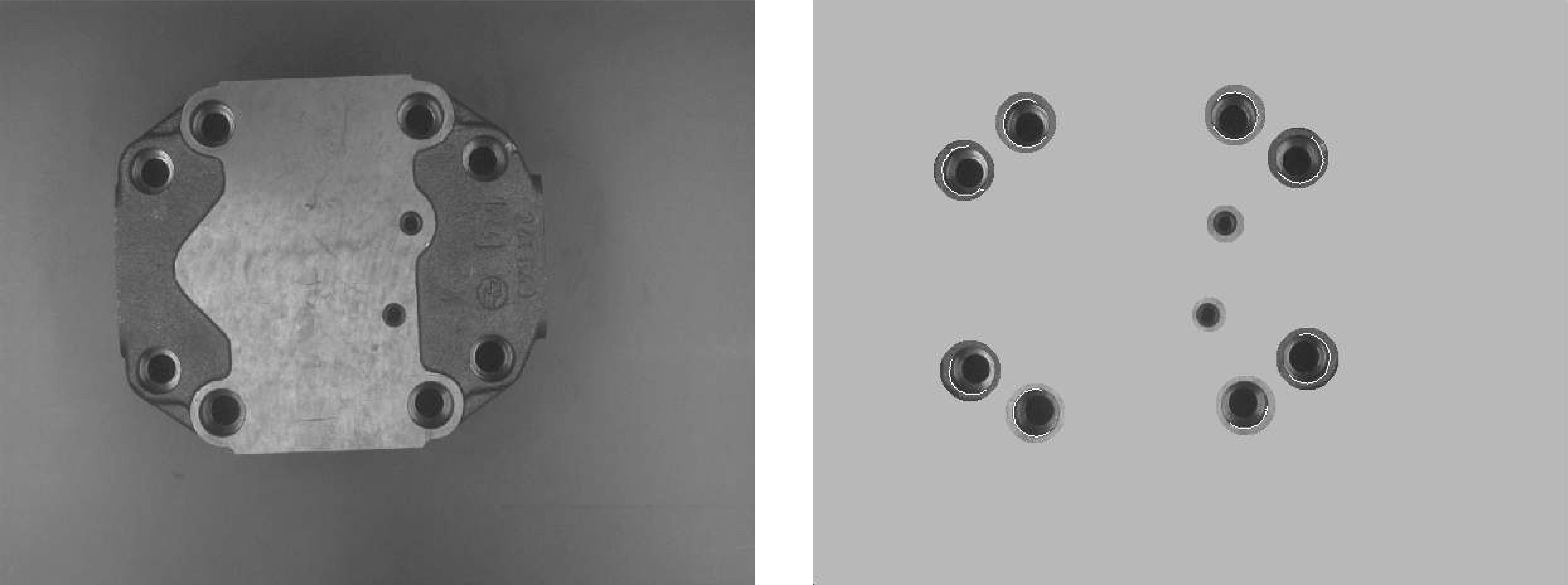
Figure 19: ROI for circle fitting: original image of a pump (left), ROI and extracted circular contours (right) -
Fit circles to the circular contour segments.
Since the final contours are all circular, the best fitting circle is calculated for each contour bycount_obj (SortedContours, NumSegments) for i := 1 to NumSegments by 1 select_obj (SortedContours, SingleSegment, i) NumCircles := NumCircles + 1 fit_circle_contour_xld (SingleSegment, 'atukey', -1, 2, 0, 5, 2, Row, \ Column, Radius, StartPhi, EndPhi, PointOrder) gen_circle_contour_xld (ContCircle, Row, Column, Radius, 0, rad(360), \ 'positive', 1)fit_circle_contour_xld. If also linear contours were contained in the set of contours, the circular segments have to be extract first.The best fitting circles are now generated by
gen_circle_contour_xld. -
Calculate the deviation of the circular contour segments from the fitted circles.
To get the deviation of the contour from the generated ellipses or circles in this case, the operatordist_ellipse_contour_xld (SingleSegment, 'algebraic', -1, 0, Row, \ Column, 0, Radius, Radius, MinDist, MaxDist, \ AvgDist, SigmaDist) endfordist_ellipse_contour_xldis applied. Only the deviation between the fitted circle and the contour segment used for the fitting is calculated.The quality of the fitting in relation to the real circle also depends on the coverage of the circle by the contour segment.
Inspecting a ball grid array (BGA)🔗
The example program %HALCONEXAMPLES%\solution_guide\2d_measuring\inspect_bga shows how the balls of a BGA can be checked for deformations and their correct positions in the grid. The latter is realized by comparing them with the balls of a reference BGA.
A BGA consists of very small objects, which have an approximately symmetrical gray value distribution, and for which the transition area between fore- and background can be rather large compared to the region of the object.
Because the standard region or contour-based approaches work with hard transitions, for symmetric objects with a large transition area it is recommended to extract object features with an approach that considers the gray value features instead.
More info
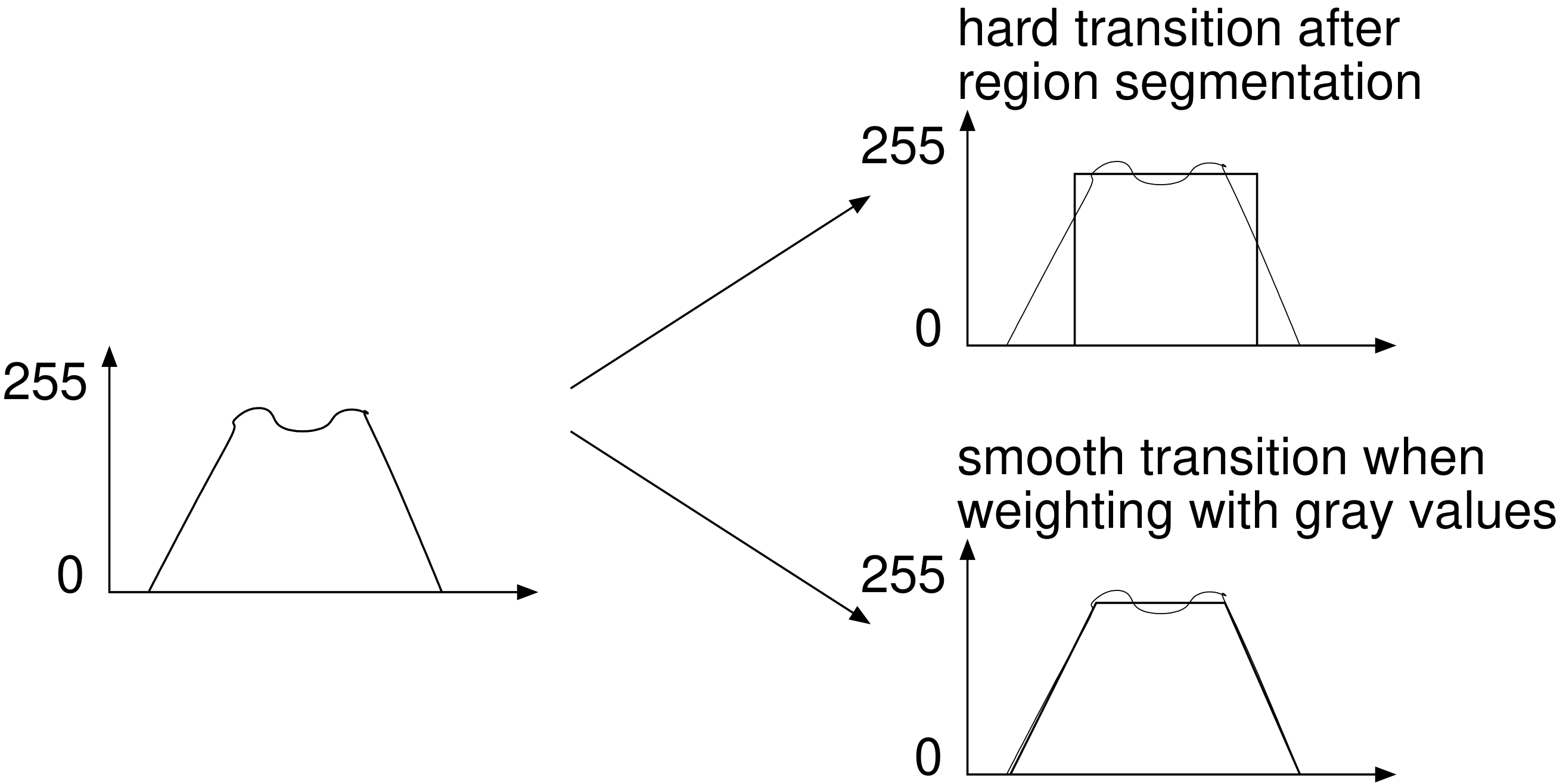
Available operators for this operation are:
area_center_gray, used to check the gray value volume and center position of each ballelliptic_axis_gray, returns the length of the axes and the orientation of the ellipse having the same orientation and aspect ratio as the input region
Steps within the example:
-
Extract balls in the reference BGA and determine their positions.
Starting with the extraction of the balls from the reference image via a region processing. Often, an additional gray value scaling is recommended, which adapts the gray value distribution according to two thresholds that depend on the fore- and background of the balls. If necessary,fast_threshold (Image, Region, 95, 255, 3) connection (Region, ConnectedRegions) select_shape (ConnectedRegions, SelectedRegions, ['area', 'anisometry'], \ 'and', [20, 1.0], [100, 1.7]) dilation_rectangle1 (SelectedRegions, RegionDilation, 3, 3) area_center_gray (RegionDilation, Image, Volume, Row, Column)area_center_graycomputes the gray value volume, the sum of the gray values of all pixels of the region, and the position of the region’s center of gravity.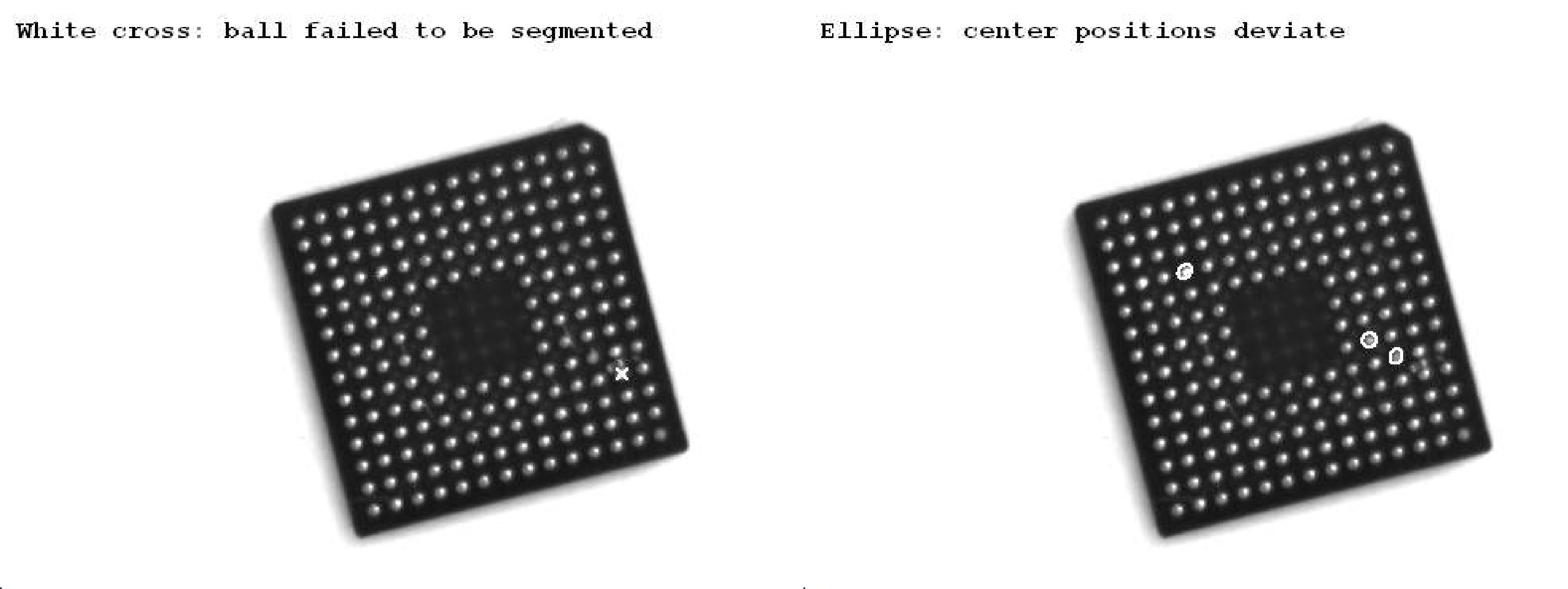
Figure 21: Irregularities of a BGA: missing ball marked by a cross (left), balls with center positions that deviate from the reference positions marked by ellipses (right) -
Sort the balls of the reference BGA.
The obtained center positions of the balls (Row,Column) are returned in an arbitrary order: The index of a variable does not contain information about the position of the corresponding ball in the grid.
To compare the center positions of corresponding balls in different BGAs, a comparable sequence of the balls is needed. This is achieved by spatially sorting the balls.More info
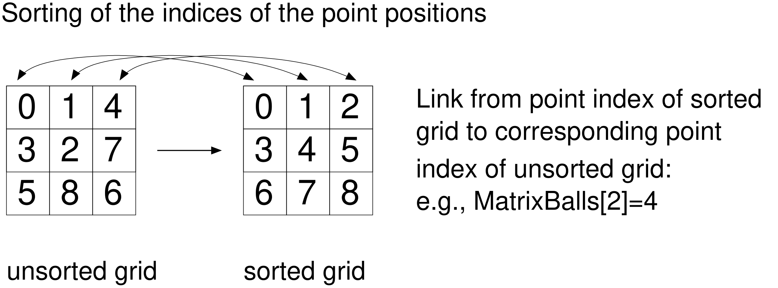
Figure 22: Sorting of the point indices To determine their positions in the grid separately for the rows and columns, we normalize the BGA as follows: We use
gen_region_pointsto create a region described by the center points of the balls and use its enclosing rectangle (obtained bysmallest_rectangle2, see Figure 22 left) to define a transformation matrix.gen_region_points (RegionBGACenters, Row, Column) smallest_rectangle2 (RegionBGACenters, RowBGARect, ColumnBGARect, \ PhiBGARect, Length1BGARect, Length2BGARect) BallsPerRow := 14 BallsPerCol := 14 BallDistCol := 2 * Length1BGARect / (BallsPerCol - 1) BallDistRow := 2 * Length2BGARect / (BallsPerRow - 1) hom_mat2d_identity (HomMat2DIdentity) hom_mat2d_rotate (HomMat2DIdentity, -PhiBGARect, RowBGARect, ColumnBGARect, \ HomMat2DRotate) hom_mat2d_translate (HomMat2DRotate, -RowBGARect + Length2BGARect, \ -ColumnBGARect + Length1BGARect, HomMat2DTranslate) hom_mat2d_scale (HomMat2DTranslate, 1 / BallDistRow, 1 / BallDistCol, 0, 0, \ HomMat2DScale) affine_trans_point_2d (HomMat2DScale, Row, Column, RowNormalized, \ ColNormalized) BGARowIndex := round(RowNormalized) BGAColIndex := round(ColNormalized)With it, the balls transform so that the grid becomes horizontal, the center position of the ball in the upper left corner is placed in the origin of the coordinate system, and the distance between the individual balls becomes
1.The rounded values for the transformed ball positions then describe the indices of the ball’s positions separately for the rows and columns of a regular grid.
Instead of separate lists for the rows and columns, a single sorted list of indices is obtained, which is ordered consecutively from left to right and from top to bottom. Therefore, a tuple is being created that has the capacity for all grid points of the BGA
BallMatrix. Its size is defined by the maximum numbers of balls per row and column.Because the actual balls of the BGA are not placed all over this grid, we first assign the start value
-1to all instances. With the help of the indices that we have obtained separately for the rows and columns of the extracted balls,BGARowIndexandBGAColIndex, we sort the balls by assigning new values to the corresponding instances ofBallMatrix.After the sorting, the value of
BallMatrixwith the index of a point coordinate in the sorted grid returns either the index of the corresponding point coordinate in the unsorted grid, or the value-1if the grid position is not occupied by a ball.NumBalls := |Row| BallMatrix := gen_tuple_const(BallsPerRow * BallsPerCol,-1) for i := 0 to NumBalls - 1 by 1 BallMatrix[BGARowIndex[i] * BallsPerCol + BGAColIndex[i]] := i endfor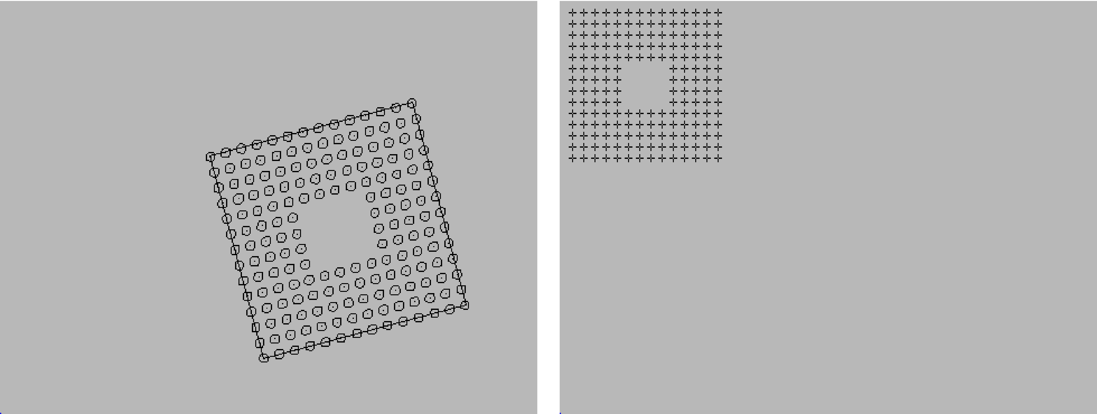
Figure 23: Normalization of the grid for the reference BGA: Smallest rectangle enclosing the region that is built by the center points of the balls (left), transformed and normalized grid (right) -
Extract balls in a second BGA and sort them according to the reference.
A second image is processed, which contains the BGA needed to be checked for irregularities. To enlarge the regions of the extracted balls useelliptic_axis_gray (RegionDilation, Image, RaCheck, RbCheck, PhiCheck) AnisometryCheck := RaCheck / RbCheckarea_center_grayandelliptic_axis_grayto get the features of the regions under consideration of their gray values.elliptic_axis_grayreturns the radii and orientation of the ellipse having the same moments as the region. The center points obtained byarea_center_grayare transformed and sorted like the center points of the reference image.Except for the additional application of
elliptic_axis_grayand an anisometry check, which are both needed to investigate the balls in a later step, the processing is the same as for the reference BGA.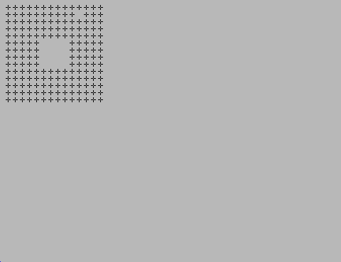
Figure 24: Transformed and normalized grid of the BGA to be checked -
Inspect the second BGA and compare it to the reference BGA
The BGA of the second image is evaluated further. Until now, there are only links from the point indices in the sorted grid to the point indices in the unsorted grid.j := 0 for i := 0 to BallsPerRow * BallsPerCol - 1 by 1 if (BallMatrix[i] >= 0 and BallMatrixCheck[i] >= 0) Rows1[j] := Row[BallMatrix[i]] Cols1[j] := Column[BallMatrix[i]] Rows2[j] := RowCheck[BallMatrixCheck[i]] Cols2[j] := ColumnCheck[BallMatrixCheck[i]] Phi2[j] := PhiCheck[BallMatrixCheck[i]] Ra2[j] := RaCheck[BallMatrixCheck[i]] Rb2[j] := RbCheck[BallMatrixCheck[i]] Anisometry2[j] := AnisometryCheck[BallMatrixCheck[i]] Volume2[j] := VolumeCheck[BallMatrixCheck[i]] j := j + 1 endif endforCreate tuples, that contain the actual data of the existing balls in the specified order, for the row and column coordinates of the balls in the reference BGA
Rows1andCols1and in the BGA to be checkedRows2andCols2. Also for the ellipse radiiRa2andRb2, anisometry valuesAnisometry2, and the gray value volumesVolume2of the second BGA are created.These tuples are reduced sets of data as they contain only the data for the grid positions that are occupied by balls in both BGAs. The size of the tuples is related to the actual number of extracted balls in the second image and not to the number of possible grid positions.
To compare the center positions of the balls of the second BGA with the center positions of the balls of the reference BGA, by superimposing both sets of positions, the balls of the reference BGA are transfored, so that they have the same position, orientation, and scale as the corresponding balls of the BGA to be checked.
For the superimposition, the operator
vector_to_rigiddetermines the affine 2D transformation by the point correspondences between both sets of coordinates.With the obtained transformation matrix, the reduced set of positions for the reference BGA (
Rows1,Cols1) is transformed intoRowTransandColumnTrans.To check also for missing balls in the second BGA, the set of unsorted reference positions originally obtained by
area_center_grayis transformed further. This is the set that still contains all positions of the regular grid, including the positions that regularly do not contain balls, marked by the value-1inBallMatrixand the positions of the balls that are only detected in the reference BGA.vector_to_rigid (Rows1, Cols1, Rows2, Cols2, HomMat2D) affine_trans_point_2d (HomMat2D, Rows1, Cols1, RowTrans, ColumnTrans) affine_trans_point_2d (HomMat2D, Row, Column, RowTransFull, ColumnTransFull)Then, the distance between the sorted points of the BGA to be checked (
Rows2,Cols2) and the sorted and transformed points of the reference BGA (RowTrans,ColumnTrans) is calculated bydistance_pp (Rows2, Cols2, RowTrans, ColumnTrans, Distance)Now, the complete grid is investigated again. For each position of the regular grid, the existence of a corresponding ball in both BGAs is checked.
If the grid position contains a ball in both sets, with both indices are larger than
-1, the sorted and reduced sets of data can be used for the comparison.The distance between the corresponding center positions is queried:
- If it is larger than 0.05 pixels, the ellipse for the ball is stored in the tuple
Deviation. - If it is smaller than 0.05 pixels, further features are checked, in particular the anisometry, that is, the deformation of the circle ellipse for deformed ball stored in
Deformation, and the range of the gray value volume, ellipse for outlier stored inVolume. - If a ball exists in the reference BGA but not in the BGA to be checked, a cross at the ball’s position is created (
gen_cross_contour_xld) and stored in the tupleMissing. The different results can then be visualized.
j := 0
for i := 0 to BallsPerRow * BallsPerCol - 1 by 1
    if (BallMatrix[i] >= 0 and BallMatrixCheck[i] >= 0)
        gen_ellipse (Ellipse, Rows2[j], Cols2[j], Phi2[j], Ra2[j], Rb2[j])
        if (Distance[j] > 0.05)
            concat_obj (EllipseDeviation, Ellipse, EllipseDeviation)
        else
            if (Anisometry2[j] > 1.2)
                concat_obj (EllipseDeformation, Ellipse, EllipseDeformation)
            else
                if (Volume2[j] < 5500 or Volume2[j] > 10000)
                    concat_obj (EllipseVolume, Ellipse, EllipseVolume)
                else
                    concat_obj (EllipseCorrect, Ellipse, EllipseCorrect)
                endif
            endif
        endif
        j := j + 1
    else
        if (BallMatrix[i] >= 0)
            gen_cross_contour_xld (Cross, RowTransFull[BallMatrix[i]], \
                                   ColumnTransFull[BallMatrix[i]], 10, \
                                   0.785398)
            concat_obj (Missing, Cross, Missing)
        endif
    endif
endfor
Note
The operators considering the gray value features are more precise than the corresponding operators for regions or contours. However, since their calculation is rather complex, they are only recommended for very small symmetric objects.
- If it is larger than 0.05 pixels, the ellipse for the ball is stored in the tuple
Extracting contours from color images🔗
Some features may only be detected when working with color images instead of gray value images, since they have the same gray value but a different color.
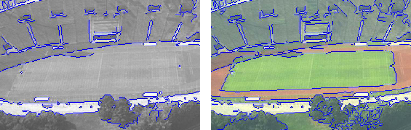
When extracting edges or lines from color images, three operators are available:
edges_color_sub_pixextracts subpixel-precise edges directly from your color image.edges_colorextracts pixel-precise edges directly from your color image.lines_coloris the suitable operator for thin linear structures like those described beforehand, but in a color image. It works similar to the approach described for gray value images, but with a more limited number of attributes that can be stored with the lines.
Examples for the contour extraction using color are:
%HALCONEXAMPLES%\hdevelop\Filters\Edges\edges_color_sub_pixfor the subpixel-precise edge extraction using color,%HALCONEXAMPLES%\hdevelop\Filters\Edges\edges_colorfor the pixel-precise edge extraction using color%HALCONEXAMPLES%\hdevelop\Filters\Lines\lines_colorfor the extraction of thin linear structures using color