Optimization🔗
Identify corresponding object parts🔗
In many applications, similar objects must be measured and the results must be compared to the results obtained for a reference image or reference data stored in a Computer Aided Design (CAD) model.
You can import ARC/INFO or DXF files via read_contour_xld_arc_info or read_contour_xld_dxf.
If you wish to create an image containing the CAD model you can create an artificial image by gen_image_const and paint the contour of the CAD model into it using paint_xld.
To identify errors of an object, like a specific drill hole that is missing, the corresponding parts of the measured object and the reference object must be clearly identified.
The example program %HALCONEXAMPLES%\solution_guide\2d_measuring\ measure_metal_part_id measures the drill holes of metal parts.
The first image is used as reference image.
The program detects missing drill holes as well as drill holes that deviate more than 2 pixels in their center position or radius from the corresponding drill holes of the part in the reference image.
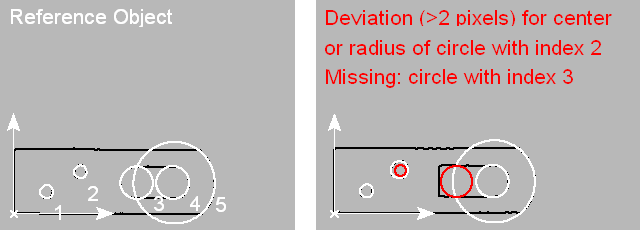
The general steps of the program are:
-
Extract and rotate contours to get a horizontal object
For each image, an ROI for the following contour processing is created. To do so, the region of the object is obtained with
threshold, the region is enlarged withdilation_rectangle1, and the image is reduced to this region byreduce_domain. Inside the ROI,threshold_sub_pixis applied to extract the contours of the metal part’s boundary.The metal parts can be arbitrarily positioned and oriented in the image. Thus, we rotate their contours, so that every metal part is horizontal when being inspected. To realize the rotation, for each image the orientation and center position of the object’s region are obtained by
orientation_regionandarea_center. These are used to create a transformation matrix (vector_angle_to_rigid) and the transformation matrix is used for the affine 2D transformation that rotates the contours (affine_trans_contour_xld). -
Measure
The rotated contours of each metal part are segmented into lines and circles, which are sorted according to their spatial position. The sorting of the segments is important to have the circles of the images to measure and the circles of the reference image in the same sequence. The sorted contours are now used to find the best-fitting lines and circles for the segments. The circle data is the actual feature we want to obtain for each image and which we want to compare to the results of the reference image.
-
Create object coordinate system
The lines are now used to create an object coordinate system with the lower left corner of the horizontal metal part as origin. The axes are built by the vertical line on the left border and the horizontal line at the lower border of the metal part. To do so, first all horizontal and vertical lines are separated by selecting the lines with a specific direction. Then, we determine the row and column coordinates of the horizontal line with the highest row coordinate (in the image coordinate system). The intersection is done via the operator
intersection_linesand results in the point coordinatesRow0andCol0, the origin of the object coordinate system. -
Transform results into the object coordinate system
To transform the already obtained center points of the fitted circles from the image coordinate system into the object coordinate system, we create a transformation matrix. Because the coordinates of the image coordinate system are seen from left to right and from top to bottom, and we want the local coordinate system seen from left to right but from bottom to top, we horizontally mirror the coordinate system by adding a slant of 180° to the transformation matrix using the operator
hom_mat2d_slant. Because the local coordinate system is parallel to the image coordinate system, no rotation is necessary, but we add a translation byhom_mat2d_translateso that Row0 and Col0 describe the new origin. The final affine 2D transformation is now applied to the positions of the circle centers, so that the actual results of the measurement are available in the local coordinate system. The transformation of the results is done viaaffine_trans_pixel. -
Store the results for the first image as reference
For the first image, we store the results so that we have them still available as reference when measuring the metal parts of the other images.
-
Compare the results for other images to the reference image
For the comparison of the reference image with the image to measure, we first check whether the number of obtained circles is equal. If so, we check for small deviations of the positions or radii between the corresponding circles. To check the deviation, the distance between the center points of the circles are determined by
distance_ppand the difference between the circle radii is computed. If at least one of them is bigger than 2 pixels, the deviating circles are marked in the image. If the number of circles in both images are not equal, the sorted circles are compared with each other. In particular, each result of the image to measure is compared to the result of the reference image having the same index, this is the reason for sorting the segments at the beginning of the contour processing. If the position and the radius allow us to conclude that the circle is the same in both images, the deviation for both is less than 10 pixels, it is checked for deviations that are larger than 2 pixels. If the deviations of position and radius are larger than 10 pixels, we assume that the circle is not the same.Then, we compare the same circle of the image to measure with the circle of the reference image having the next higher index. This procedure continues until either the corresponding circle is found or all remaining circles of the reference image were checked.
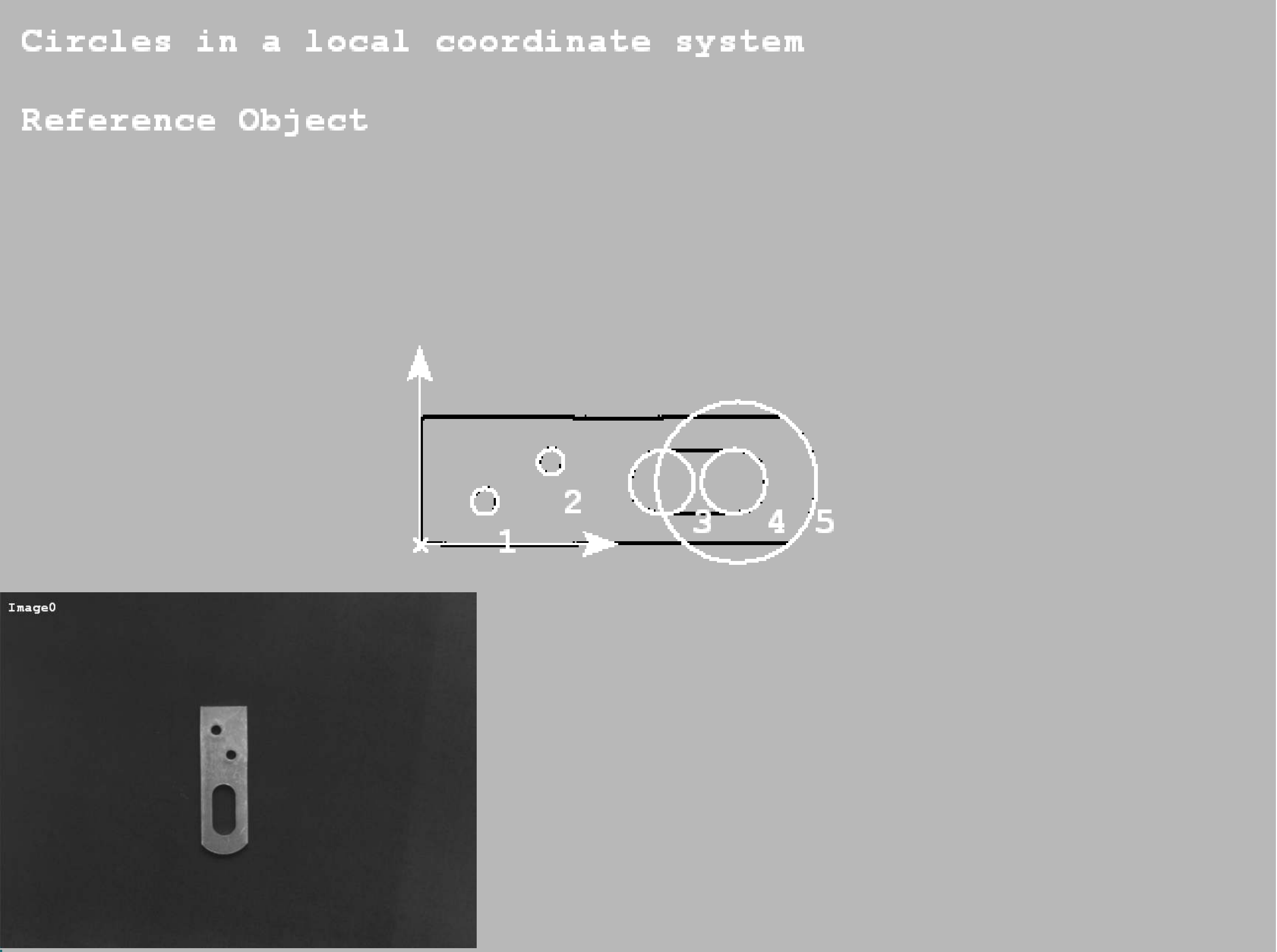
Figure 2: Comparison of the circle data to the circle data of a reference image
Measure in world coordinates🔗
In many applications, the dimensions of the measured objects must be determined in world coordinates, for example, in μm. A second reason for measuring in world coordinates is to compensate radial and perspective distortions. For measuring in world coordinates, a camera calibration must be applied. It results in the exterior camera parameters, data describing the relation of the camera to the plane in which the 2D measurements are realized.
With the obtained data, two kinds of transformations can be applied:
- You can either measure the features of interest in the distorted image and afterwards transform them into the world plane
- You use the data to first transform the image and then apply your measurements in the transformed image.
Which approach to choose depends on the basic tools you use for the measuring. If you obtain your measurement results by contour processing, it is recommended to first measure and then transform the resulting points or contours into world coordinates.
To do so, after the camera calibration you apply the operators image_points_to_world_plane or contour_to_world_plane_xld.
For detailed information about how to transform image into world coordinates see Transforming image to world coordinates and vice versa.
If you measure via region processing, the transformation of results can become rather complex, so it is recommended to first transform or rectify the image and then measure in the transformed image. For detailed information about rectifying images, we recommend to read Rectifying images.
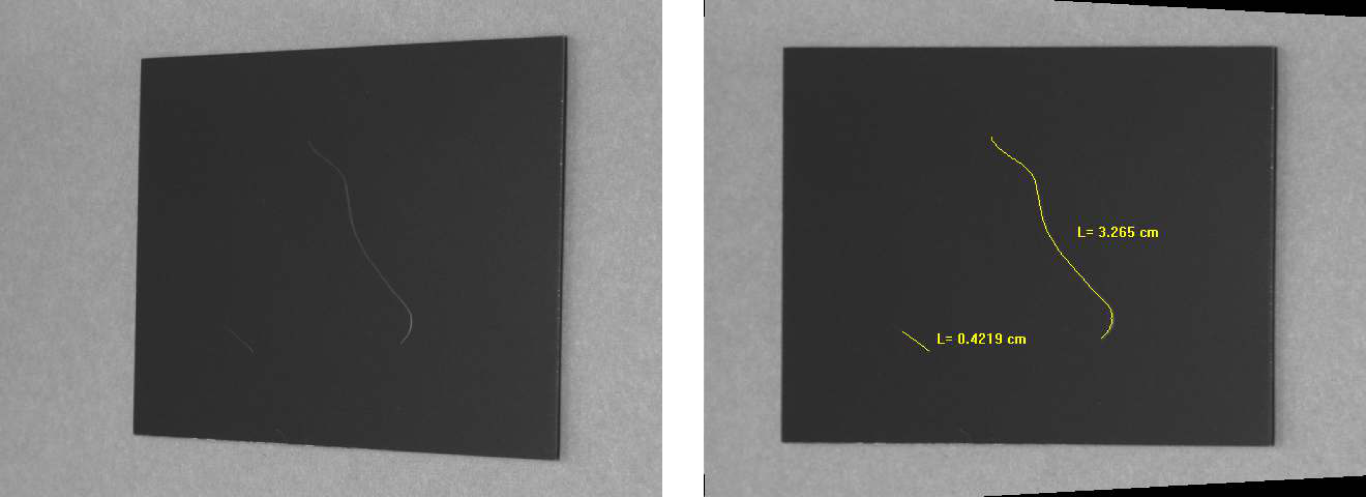
The example program %HALCONEXAMPLES%\solution_guide\2d_measuring\measure_perspective_scratch measures the lengths of scratches on a planar anodized aluminum surface.
-
Calibrate the camera
The example starts with the camera calibration (see Camera calibration). For this, multiple images are needed, each containing a calibration plate that is placed in a different position and orientation. In one of the calibration images, in this case in the first one, the calibration plate must be placed in the measuring plane, it must be parallel ,with a known distance, to the anodized aluminum plate we want to investigate. To calibrate the camera, information about the used calibration plate and initial values for the internal camera parameters must be known. The information on the used standard calibration plate, the positions of the marks inside the calibration plate coordinate system, is stored in the file
caltab_30mm.descr. This and other information is added to a so-called calibration data model.In the program, the images containing calibration plates are read. For each image in the loop,
find_calib_objectsearches for the calibration plate in the image and determines the marks, calculates their 2D positions in the image, and estimates the pose of the calibration plate. The contours and point coordinates of the marks are accessed from the calibration data model withget_calib_data_observ_contoursandget_calib_data_observ_points. -
Transform the image
The pose of the measuring plane, the external camera parameters obtained for the image in which the calibration plate lies in the measuring plane, is now stored in the variable
PoseCalib. Since the calibration plate was rotated by 90° (the black triangular mark normally has to be placed in the upper left corner), we add a rotation to the corresponding parameter of the pose usingtuple_replace. Poses can be defined by different sequences of translations and rotations (see About poses).If you are not sure about the sequence used for the pose you want to change, you can also convert the pose to a homogeneous transformation matrix with
pose_to_hom_mat3d, explicitly add a local rotation to the axis you want to change usinghom_mat3d_rotate_local, and convert the resulting homogeneous transformation matrix back to a pose usinghom_mat3d_to_pose.Additionally, we apply the operator
set_origin_poseto the pose to add a translation to the z-coordinate to compensate for the distance between the calibration pattern and the measuring plane, which is described by the known thickness of the calibration plate.The translations in x- and y- direction are applied mainly so that the rectified image optimally fits the displaying window. From the corrected pose, the operator
pose_to_hom_mat3dcreates a homogeneous transformation matrix. This is used bygen_image_to_world_plane_mapto generate a projection map that describes the mapping between the image plane and the plane z=0 of a world coordinate system. This map can be used now to transform the images with the operatormap_imageso that the measuring plane is rectified with a scaling described by PixelDist.Here, we transform two images, one containing the calibration plate that is placed in the measuring plane, and the other containing the scratches we want to investigate. The first one is transformed mainly for visualization purposes, whereas the latter is the actual image we wanted to obtain. This image ( ModelImageMapped ) is used now for the actual measurement.
-
Measure in the transformed image
The measurement starts with the extraction of the aluminum plate and the following code searches for scratches having a minimum size and extent. In particular, the region of the aluminum plate is extracted using
fast_threshold,fill_upfills the remaining holes in the region, and an erosion (erosion_rectangle1) suppresses the edges of the border for the later extraction of the scratches. Inside this region, the scratches are extracted byfast_thresholdand processed by some morphological operatorsdilation_circleanderosion_circle. The obtained region is separated into connected components byconnectionand components with a specific size and extent are selected as scratches. In a loop, the individual scratches are reduced to their medial axis byskeleton. The skeletons are converted into contours bygen_contours_skeleton_xldand for each contour, the lengthlength_xldand center positionarea_center_points_xldare obtained.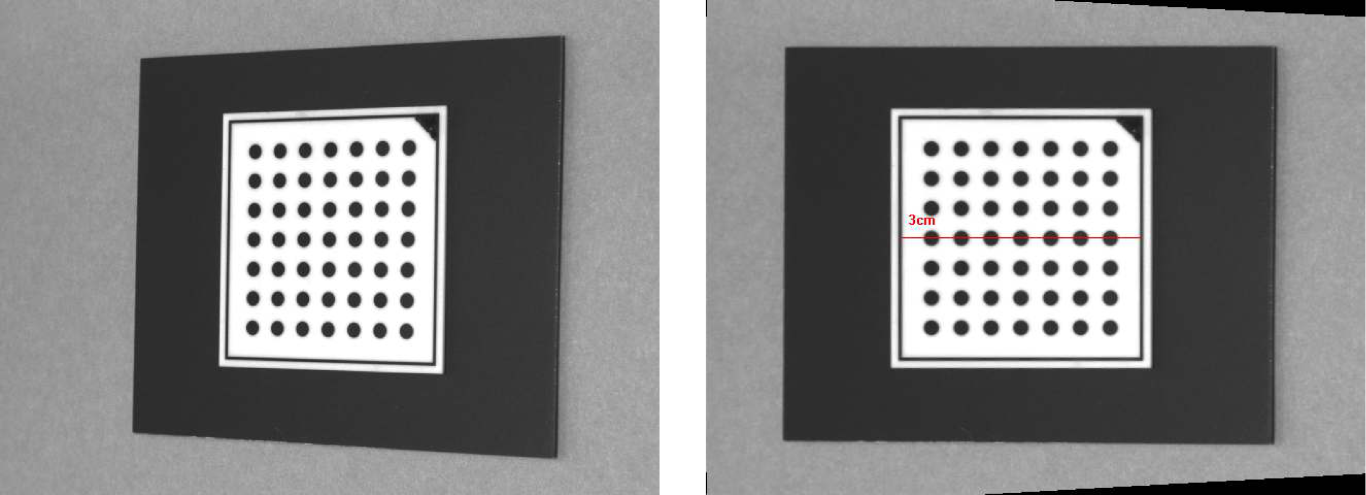
Figure 4: Calibration plate in the measuring plane: (left) perspectively distorted image, (right) image after transformation