Using measure objects🔗
Measure objects can be used for the following tasks:
- Measure position of individual edges and the distance between
- Extract edge pairs
- Determine points with particular gray values along the profile
- Access the gray value profile
- Transform object dimensions into world coordinates
Edge position🔗
The position of the individual determined edges can be measured with the operator measure_pos.
With this approach, it is also possible to extract edges that appear only if the image is smoothed in a direction perpendicular to the ROI.
In the example program %HALCONEXAMPLES%\solution_guide\1d_measuring\measure_ic_leads.hdev,
we use this operator to measure the length of the leads of the IC displayed in
Figure 1.
At a first glance,
it is not clear how to solve this task because the individual leads are not enclosed by two edges.
However, we
can exploit the averaging perpendicular to the profile line: If the ROI encloses multiple leads, as depicted in figure
Figure 1, the averaged gray value of the leads is darker
than the background, but lighter than the body of the IC (see
and
).
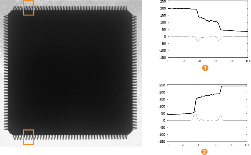
First, a measure object is created for the ROI at the top of the image. The ROI must have a width such that it contains several leads.
gen_measure_rectangle2 (Row, Column, Phi, Length1, Length2, Width, Height, Interpolation, MeasureHandle)
Now, all edges that are perpendicular to the ROI are extracted.
measure_pos (Image, MeasureHandle, Sigma, Threshold, Transition, Select, RowEdge, ColumnEdge, Amplitude, Distance)
The resulting edges enclose the leads (see Figure 2).
Their distance is returned in the parameter Distance.
In the example, only two edges are returned.
Therefore, the parameter Distance contains only one element, which is the length of the leads at the top of the image.
To determine the length of the leads at the bottom of the image, the same measurements are carried out within the second ROI.
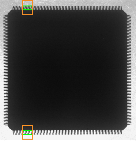
Distance \(= 27.06\) (top) and Distance \(= 32.03\) (bottom). The parameter Sigma determines the degree of smoothing of the profile along the profile line.
The parameter Threshold defines the threshold that is applied to the derivative of the profile for the selection of edges.
Both parameters are described here.
The parameter Transition can be used to select edges with a particular transition.
If Transition is set to 'negative', only edges at which the gray values change from light to dark will be returned.
In the current example, the two edges in the ROI at the top of the image have a negative transition.
If Transition is set to 'positive', only edges at which the gray values change from dark to light (for example, the two edges in the ROI at the bottom of the image) will be returned.
To determine all edges, Transition must be set to 'all' in this application.
The parameter Select can be used to restrict the result to the 'first' or 'last' edge.
In the current example, Select must be set to 'all'.
Besides the distance of the edges, measure_pos also returns their position in the output parameters RowEdge and ColumnEdge as well as their amplitude (Amplitude).
In the example, the position is used to visualize the edges:
Edge pair position🔗
Whenever the object to measure is enclosed by two edges, you can use the operator measure_pairs, which groups edges to edge pairs.
In the following example, we use this operator to determine the width of the leads from the image displayed in Figure 3.
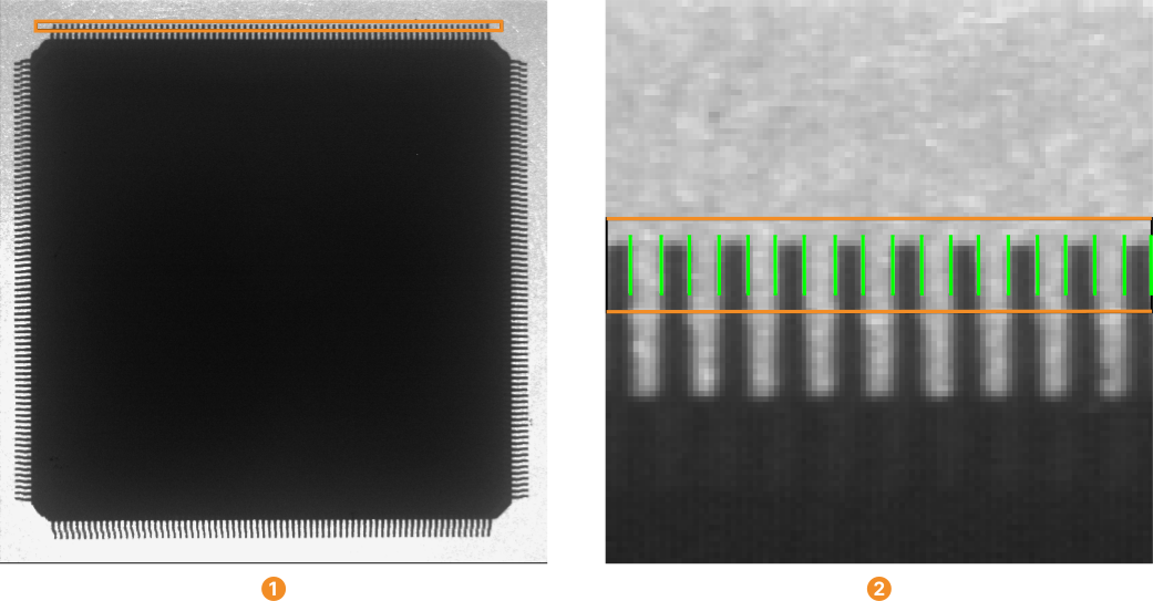
First, a suitable ROI must be defined. Because we want to determine the edges of the individual leads, the ROI must be oriented perpendicular to the leads (see ). Here, it is oriented from the left to the right. With this ROI, a measure object is created.
Now, all edge pairs that enclose dark image regions are extracted (%HALCONEXAMPLES%\solution_guide\1d_measuring\measure_ic_leads.hdev):
measure_pairs (Image, MeasureHandle, Sigma, Threshold, Transition, Select, RowEdgeFirst, ColumnEdgeFirst, AmplitudeFirst, RowEdgeSecond, ColumnEdgeSecond, AmplitudeSecond, IntraDistance, InterDistance)
The parameters of measure_pairs are partly identical to the ones of measure_pos:
Sigma determines the degree of smoothing of the profile.
The parameter Threshold defines the threshold that is applied to the derivative of the profile for the selection of edges.
The parameters are described in the section about 1D edge extraction.
The parameter Transition can be used to select edge pairs with a particular transition.
If Transition is set to 'negative', as in the example, only edge pairs where the first edge has a negative transition and the second edge has a positive transition, that is, edge pairs that enclose a dark image region will be returned.
If Transition is set to 'positive', the behavior is exactly opposite, that is, edge pairs that enclose a bright image region will be returned.
If Transition is set to 'all', the transition is determined by the first edge.
that is, dependent on the positioning of the measure object, edge pairs with a light-dark-light transition or edge pairs with a dark-light-dark transition are returned.
This is suited, for example, to measure objects with different brightness relative to the background.
If more than one consecutive edge with the same transition is found, only the first one will be used as a pair element.
This behavior may cause problems in applications in which the Threshold cannot be selected high enough to suppress consecutive edges of the same transition.
This problem can be demonstrated, for example, by defining the ROI in the example program %HALCONEXAMPLES%\solution_guide\1d_measuring\measure_switch.hdev the other way round, that is, from bottom right to top left.
Then, the first edge with a negative transition corresponds to the shadow of the pin and the edge that corresponds to the pin itself is not used as a pair element (see Figure 4
).
For these applications, an advanced pairing mode exists that only selects the strongest edges of a sequence of consecutive edges of the same transition.
This mode is selected by appending '_strongest' to any of the above modes for Transition, for example, 'negative_strongest'.
Figure 4
shows the result of setting Transition to 'negative_strongest'.
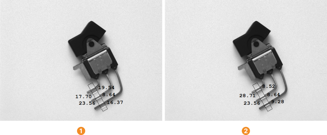
Transition = 'negative',
Transition = 'negative_strongest'. The parameter Select can be used to restrict the result to the 'first' or 'last' edge pair.
To determine all edge pairs, Select must be set to 'all'.
The operator measure_pairs returns the coordinates of the edge positions separately for the first and the second edge of each edge pair.
The output parameters RowEdgeFirst and ColumnEdgeFirst contain the coordinates of the first edges of the edge pairs and the parameters RowEdgeSecond and ColumnEdgeSecond contain the coordinates of the second edges.
With this, the center of the pairs can easily be determined by calculating the mean of the respective first and second edge positions:
RowPairCenter := (RowEdgeFirst + RowEdgeSecond) / 2.0
ColumnPairCenter := (ColumnEdgeFirst + ColumnEdgeSecond) / 2.0
The output parameters IntraDistance and InterDistance contain the distance between the two edges of the
edge pairs and the distance between the edge pairs.
Position of points with particular gray value🔗
With the operator measure_thresh, it is also possible to determine the subpixel precise positions where the gray value profile has a given value.
This 1D thresholding works like the 2D subpixel precise thresholding operator threshold_sub_pix.
This operator can be useful to extract particular edges in applications where the lighting conditions can be con- trolled very accurately. Note that the measured position depends heavily on the brightness of the image, that is, the measured position will vary if the brightness level of the image changes, for example, due to illumination changes.
Gray projection🔗
For applications that require the determination of special 1D features, it is possible to access the gray value profile directly via the operator measure_projection.
It returns the original, that is, unsmoothed gray value profile as a tuple in the output parameter GrayValues.
On the profile, points that satisfy a particular condition can be determined.
Then, the pixel coordinates of these points can be calculated.
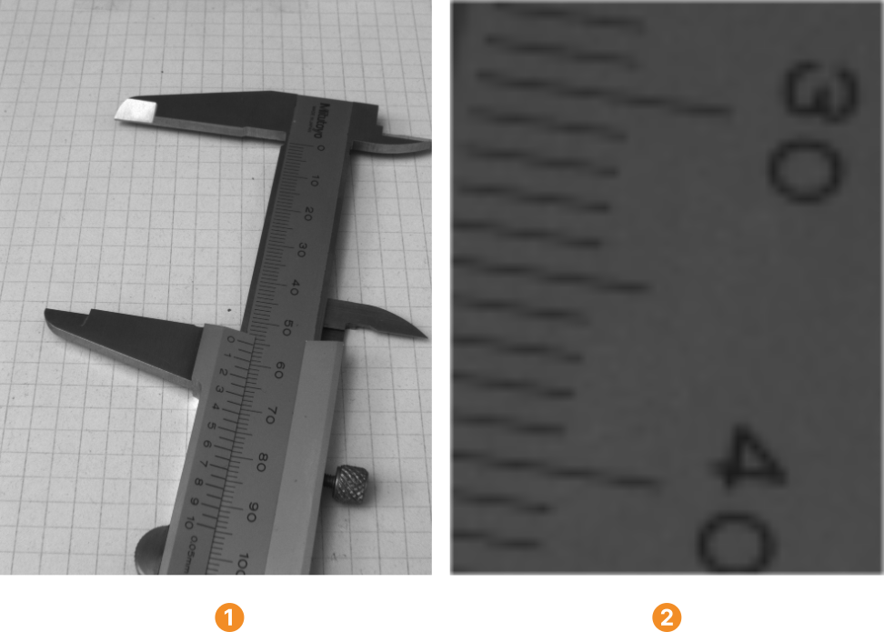
In the example program %HALCONEXAMPLES%\solution_guide\1d_measuring\measure_caliper.hdev, the distances between the pitch lines of a caliper are determined.
The used image (Figure 5
) shows the pitch lines as approximately one pixel wide lines (see, for example, Figure 5
).
To determine the line positions in the gray value profile, a 1D line extraction is implemented based on the gray value profile.
First, the measure object is created. It is positioned such that only the longest pitch lines, that is, those which indicate full centimeters run through the measuring ROI
gen_measure_rectangle2 (Row, Column, Phi, Length1, Length2, Width, Height, 'bilinear', MeasureHandle)
Then, the profile is determined with the operator measure_projection, which returns the profile in the output parameter GrayValues:
To reduce the noise, the profile must be smoothed because the operator measure_projection returns the original, that is, unsmoothed profile.
Sigma := 0.3
create_funct_1d_array (GrayValues, Function)
smooth_funct_1d_gauss (Function, Sigma, SmoothedFunction)
The smoothed profile is displayed in Figure 6.

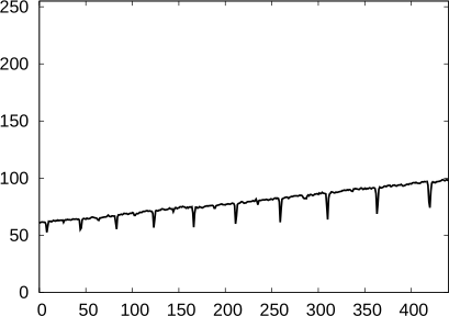
To detect line points on the profile, it is sufficient to determine the points where the first derivative of the smoothed profile vanishes.
The first derivative of the smoothed profile is determined with the operator derivate_funct_1d with the control parameter Mode set to 'first'; the points where the first derivative vanishes are determined with the operator zero_crossings_funct_1d:
derivate_funct_1d (SmoothedFunction, 'first', FirstDerivative)
zero_crossings_funct_1d (FirstDerivative, ZeroCrossings)
The first derivative of the smoothed profile is displayed in []#fig-mvtasks-method-measure-1d-measure_objects_usage-gray_projection-profile_derivatives) .

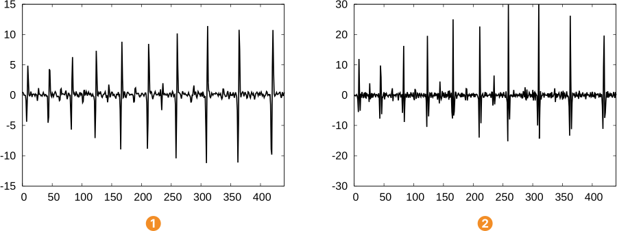
Because of noise, the first derivative shows many more zero crossings than just in the middle of each line, that is, between the large negative and positive spikes in Figure 7
.
We can select the desired zero crossings by looking at the magnitude of the second derivative: Bright lines on a dark background will have a negative second derivative while dark lines on a bright background will have a positive second derivative.
The second derivative of the smoothed profile is determined with the operator derivate_funct_1d with the control parameter Mode set to 'second':
In our case, the pitch lines appear as dark lines on a bright background.
Therefore, we have to select those line positions, where the second derivative has a large positive value: For each line position, that is, zero crossing of the first derivative, the value of the second derivative is determined with the operator get_y_value_funct_1d.
If this value is larger than a user defined threshold, the line position will be stored in a tuple that holds the positions of all salient lines.
MinimumMagnitudeOfSecondDerivative := 8
PositionOfSalientLine := []
for i := 0 to |ZeroCrossings| - 1 by 1
    get_y_value_funct_1d (SecondDerivative, ZeroCrossings[i], 'constant', Y)
    if (Y > MinimumMagnitudeOfSecondDerivative)
        PositionOfSalientLine := [PositionOfSalientLine,ZeroCrossings[i]]
    endif
endfor
Finally, the positions of the lines on the profile must be transformed into pixel coordinates because measure_projection returns just the gray value profile along the profile line.
Note that internally, the coordinates of the center of the measuring ROI are rounded and the length of the measuring ROI is set to the largest integer value that is smaller or equal to the given value.
The pixel coordinates of the start point of the profile line can be determined as follows (see Figure 8)
This can be realized by the following lines of code:
RowStart := floor(Row + 0.5) + floor(Length1) * sin(Phi)
ColStart := floor(Column + 0.5) - floor(Length1) * cos(Phi)


Now, the pixel coordinates of the positions of the salient lines on the profile can be determined as follows:
This can be expressed by the following lines of code:
RowLine := RowStart - PositionOfSalientLine * sin(Phi)
ColLine := ColStart + PositionOfSalientLine * cos(Phi)
Figure 9 shows the positions of the determined lines.
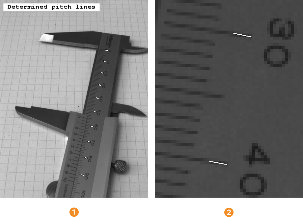
In the following section, the pixel coordinates of the pitch lines and the distance between them are transformed into world coordinates.
If you are using a circular measure object, which has been created with the operator gen_measure_arc, the
following formulae must be used to determine the pixel coordinates RowPoint and ColPoint of a point on the
profile:
Here, Position is the position of the point on the profile and CenterRow, CenterColumn, Radius, and AngleStart are the parameters used for the creation of the measure object with the operator gen_measure_arc.
Measuring in world coordinates🔗
In many applications, the dimensions of the measured object must be determined in world coordinates, for example, in μm. This can either be achieved by transforming the original measurement results into world coordinates or, by first rectifying the image and applying the measurement in the transformed image. As a prerequisite, the camera must be calibrated.
In the example program %HALCONEXAMPLES%\solution_guide\1d_measuring\measure_caliper.hdev, first the positions of the pitch lines of a caliper are determined.
These positions are now transformed into world coordinates with the operator image_points_to_world_plane:
The parameter CamParam contains the camera parameters and the parameter WorldPose the position and orientation of the world plane in which the measurement takes place.
Both parameters can be determined during the camera calibration.
In the current example program, they are assumed to be known.
Now, the distance between the pitch lines can be calculated with the operator distance_pp:
The resulting distances are displayed in Figure 10.
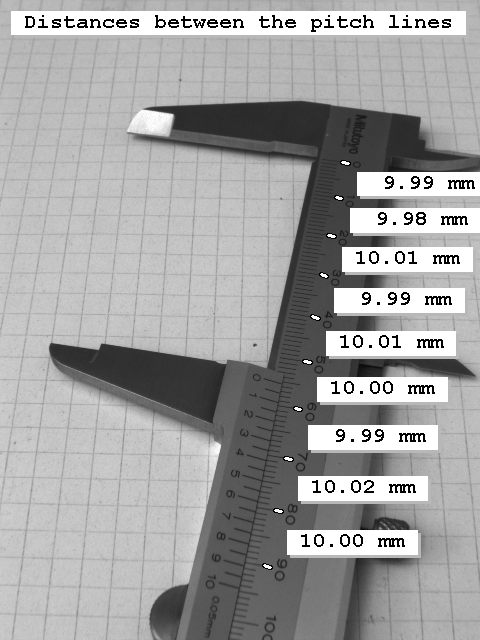
Tips and tricks🔗
Distances for circular ROIs🔗
There are multiple representations for the distance between two edges that are determined with a measure object that is based on a circular ROI (see Figure 11):
arc length
linear distance
angular distance


Measure objects based on a circular ROI return the distances as arc lengths.
The example program %HALCONEXAMPLES%\solution_guide\1d_measuring\measure_ring.hdev shows that it is very easy to transform the measurements into another representation.
In this example, the size of the cogs of a cogwheel must be measured (see Figure 12).
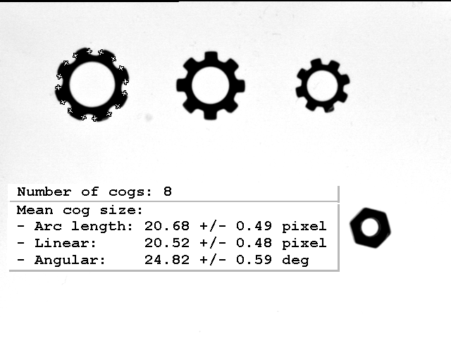
First, a measure object is created based on a circular ROI:
gen_measure_arc (CenterRow, CenterCol, Radius, AngleStart, AngleExtent, AnnulusRadius, Width, Height, Interpolation, MeasureHandle)
Then, the edges of the cogs are determined with the operator measure_pairs:
measure_pairs (Image, MeasureHandle, Sigma, Threshold, Transition, Select, RowEdgeFirst, ColumnEdgeFirst, AmplitudeFirst, RowEdgeSecond, ColumnEdgeSecond, AmplitudeSecond, IntraDistance, InterDistance)
The size of the cogs, that is, the distance between the edges of the edge pairs is returned in the output parameter IntraDistance as arc length.
The linear distance can be calculated from the coordinates of the edges with the operator distance_pp:
The angular distance can be derived from the arc lengths as follows:
which is implemented in the example program as follows:
Note that here the angular distance is determined in degrees.
ROIs partially outside the image🔗
Gray value information exists only for positions on the profile line where at least a part of the respective line of projection lies inside the image. If parts of an ROI lie outside the image, the edges inside the image and the distances between them will still be determined correctly.
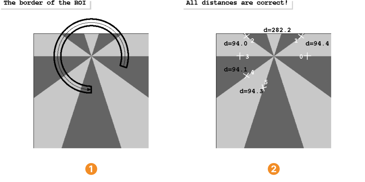
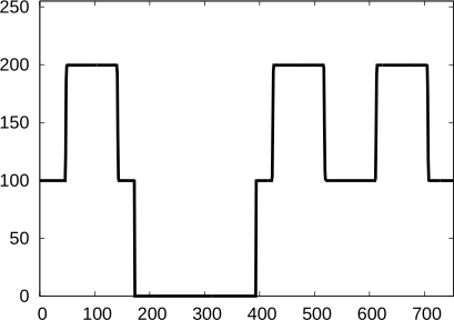
The example presented in Figure 13 demonstrates such a case. Here, the edges of a Siemens star must be determined with a measure object centered at the center of the Siemens star. In , the image as well as the outline of the ROI are shown. The upper part of the ROI lies outside the image. The distances between the edges as returned by the measure object are displayed in .
Note that at positions where no gray value information is available, the profile contains zeros. Figure 3.14 shows the gray value profile determined with the operator measure_projection from the measure object that was created with the above described circular ROI (see ).

Accuracy vs. speed🔗
By default, the averaging of gray values is performed using fixed point arithmetic, to achieve maximum speed.
You can trade some of the speed against accuracy by setting the system parameter 'int_zooming' to 'false' with the operator set_system.
Then the internal calculations are performed using floating point arithmetic.
Note that the gain in accuracy is minimal.
See also the description of the parameter Interpolation.