GMM classification🔗
Gaussian mixture models (GMM)🔗
Classification with Gaussian mixture models (GMM) is based on the Bayes decision rule.
Generally, the Bayes decision rule minimizes the probability of incorrectly classifying a feature vector by assigning it to the class with the highest a posteriori probability.
The Bayes decision rule partitions the feature space into mutually disjoint regions. The regions are separated by decision boundaries, which can be points for one-dimensional data, curves for two-dimensional data, or hypersurfaces for higher-dimensional data. The boundaries are defined by points where neighboring classes have the same probability.
The Bayes decision rule can be expressed as
where
- \(x\) is the feature vector,
- \(w_i\) denotes class \(i\),
- \(P(w_i)\) is the prior probability of class \(i\),
- \(P(x \mid w_i)\) is the conditional probability of observing \(x\) given class \(i\), and
- \(P(w_i \mid x)\) is the posterior probability that \(x\) belongs to class \(i\).
For a given feature vector \(x\), \(P(x)\) is constant for all classes and therefore does not influence the classification decision. Thus, the classification can equivalently be based on
The class with the highest posterior probability is selected.
Estimation of class probabilities🔗
The first problem of the Bayes classifier is how to obtain \(P(w_i)\), the probability of occurrence of a class.
Two strategies can be followed:
-
Estimation from training data:
The class probabilities can be estimated from the training data. This is only recommended if the training set is representative not only with regard to the quality of the samples but also with regard to the frequency of the individual classes.
-
Uniform distribution:
All classes are assumed to be equally probable. In this case,
\[ P(w_i)=\frac{1}{m}, \]where \(m\) is the number of classes.
This is the preferred approach in most cases.
Estimation of conditional probabilities🔗
The second problem is how to obtain the conditional probability \(P(x \mid w_i)\).
One possibility is to estimate the probability from a histogram of the training samples. However, the number of required histogram bins grows exponentially with the feature dimension. This leads to the so-called curse of dimensionality.
Another approach is k-nearest-neighbor density estimation. Here, the number of samples is kept constant while the volume of the region containing these samples is varied. However, all training samples have to be stored with the classifier and finding the nearest neighbors is computationally expensive. Therefore, this approach is seldom used in practice.
A practical approach is to assume that \(P(x \mid w_i)\) follows a known distribution, such as a normal distribution. In this case, the mean vector and covariance matrix of the distribution have to be estimated.
Gaussian mixture model representation🔗
In some cases, a single normal distribution is not sufficient to represent the variations within a class.
For example, a class can contain samples with significantly different feature values while all samples still belong to the same class. In such cases, several distributions may be required to represent the class.
If these distributions are assumed to be normally distributed, their combination results in a Gaussian mixture model.
During training, the parameters of the Gaussian mixture model are estimated using the Expectation Maximization (EM) algorithm. During classification, the posterior probabilities of the individual classes are evaluated and the sample is assigned to the most probable class.
A GMM classifier represents the probability density of each class as a linear combination of Gaussian distributions. Figure [Gaussian distributions within a class][fig-gmm-distributions] illustrates how multiple Gaussian distributions can represent the variations within a class.
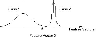
Figure 1. Gaussian distributions within a class.
The covariance of the Gaussian distributions determines the shape and orientation of the modeled distributions. Figure [Covariance ellipsoids representing class distributions][fig-gmm-ellipsoids] illustrates how the feature vector can be evaluated with respect to the modeled class distributions rather than only by its distance to the class centers.
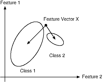
Figure 2. Ellipsoids representing Gaussian components.
GMM classifiers are reliable mainly for low-dimensional feature vectors, approximately up to 15 features.
Typical applications🔗
Typical applications of GMM classification include
- general feature classification,
- image segmentation, and
- novelty detection.
Novelty detection means that feature vectors that do not belong to one of the trained classes can be rejected.
Statistical and geometrical approaches🔗
Classification methods can generally be divided into statistical and geometrical approaches.
- Statistical approaches estimate posterior probabilities. GMM classifiers belong to this category.
- Geometrical approaches explicitly construct separating decision boundaries. Examples include SVM and neural-network-based classifiers.