Optimization🔗
This chapter describes the most important parameters and optimization techniques for Gaussian mixture model (GMM) classification.
In general, it is recommended to first optimize the classification quality and only afterwards optimize the runtime.
The most important parameters that influence the classification quality are
NumDimofcreate_class_gmm,NumCentersofcreate_class_gmm,CovarTypeofcreate_class_gmm,ClassPriorsoftrain_class_gmm.
If the classification generally works, the runtime can subsequently be optimized. The most important parameters for this are
CovarTypeofcreate_class_gmm,PreprocessingandNumComponentsofcreate_class_gmm.
The following sections introduce optimization tips for the most important GMM parameters. The focus is on parameters for which the setting has a significant influence on the classification quality, robustness, or runtime.
Further information about the respective operators can be found in the HALCON Reference.
Create the classifier🔗
A GMM classifier is created with
NumDim🔗
The parameter NumDim specifies the dimension of the feature vectors used for training and classification.
GMM classifiers work optimally for a limited number of features. If the classification result is not satisfying, using too many features may be one possible reason. As a rule of thumb, the number of features should not exceed approximately 15, although some applications also work with larger feature vectors.
If an application requires significantly more features, MLP, SVM, or k-NN classification may be preferable.
NumCenters🔗
The parameter NumCenters specifies the number of Gaussian centers used to model each class.
You can either specify a fixed number of Gaussian centers or a lower and upper bound. If a range is specified, the optimum number of centers is determined automatically using the Minimum Message Length (MML) criterion.
In most cases, it is recommended to specify a range for all classes. Start with a sufficiently high upper bound and use the expected number of centers as the lower bound. If the classification is successful, the range can subsequently be reduced to improve the classification speed.

Note
If training is canceled with error 3335 (Internal error while training the GMM), an unsuitable value or range for NumCenters is a possible cause.
CovarType🔗
The parameter CovarType specifies the type of covariance matrix used for the Gaussian components.
The available covariance types are
'spherical','diag', and'full'.
The covariance type determines the shape of the Gaussian components and therefore influences how flexibly the classes can be modeled.
With 'spherical', the covariance matrix is a scalar multiple of the identity matrix. The resulting Gaussian components have the same variance in all feature directions.
With 'diag', a diagonal covariance matrix is used. Different variances can be modeled for the individual features, but correlations between features are not considered.
With 'full', a full positive-definite covariance matrix is used. This also allows correlations between the individual features to be modeled.
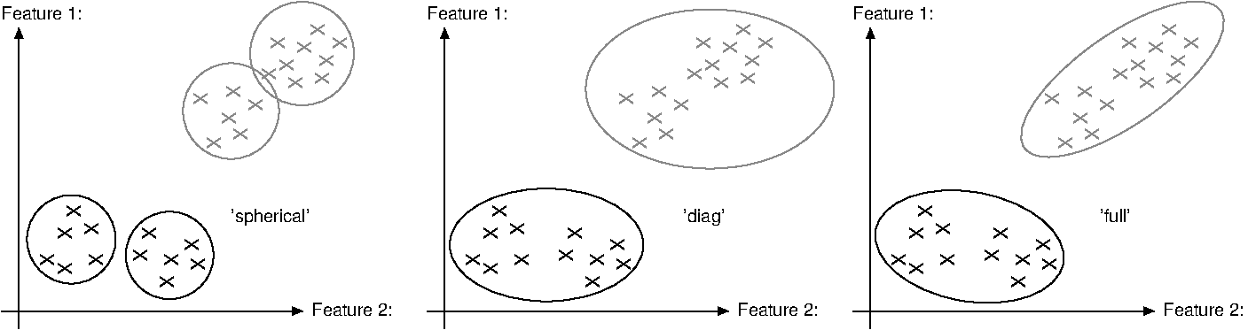
'spherical', 'diag', and 'full'. The flexibility of the classifier and the computational effort increase from 'spherical' over 'diag' to 'full'. Therefore, 'full' can model more complex class distributions, while 'spherical' is computationally less expensive.
Preprocessing🔗
The parameter Preprocessing defines the preprocessing applied to the feature vectors during training and subsequently during classification or evaluation.
The available preprocessing methods are
'none','normalization','principal_components', and'canonical_variates'.
Preprocessing can reduce the runtime of both training and classification and can sometimes also improve the classification result.
In most cases, Preprocessing should be set to 'normalization'. This usually improves the speed without losing relevant information compared to 'none'.
The values 'principal_components' and, in rare cases, 'canonical_variates' can be used to further reduce the feature dimension and thereby improve the runtime.
Therefore, Preprocessing can be used to balance classification quality and runtime. If the classification quality is already sufficient, reducing the feature dimension can be used to improve the runtime. If the classification accuracy decreases, a less aggressive preprocessing method should be selected.
NumComponents🔗
If Preprocessing is set to 'principal_components' or 'canonical_variates', NumComponents determines how many feature components are retained.
Reducing the number of components can improve the runtime of training and classification. However, choosing too few components can remove information that is relevant for the classification and therefore decrease the classification accuracy.
Therefore, NumComponents should be chosen as a trade-off between classification quality and runtime. Start with a sufficiently large number of components and reduce it while verifying the classification result on independent test data.
A suitable value for NumComponents can be determined with
Add training samples🔗
Training samples can be added using
add_sample_class_gmmfor feature vectors,add_samples_image_class_gmmfor labeled images.
The distribution of the training data strongly influences the resulting classifier. Therefore, representative training samples are essential.
Randomize🔗
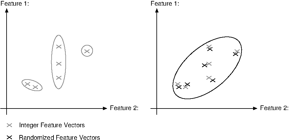
The parameter Randomize specifies the standard deviation of Gaussian noise that is added to the training data.
This parameter is mainly useful for originally integer-valued feature data. Without randomization, the modeled Gaussian distributions may become aligned with the feature axes and can result in an unnecessarily high number of Gaussian centers.
This effect can be reduced by setting Randomize to a value greater than 0.
According to experience, values between 1.5 and 2 often lead to a satisfying result.
If the feature vector was created from integer data by scaling, Randomize has to be scaled by the same scale factor that was used to scale the original data.
Train the classifier🔗
Training is performed with
MaxIter and Threshold🔗
The parameters MaxIter and Threshold control when the expectation maximization algorithm terminates.
Reducing MaxIter can improve the training speed for specific applications. However, reducing the number of iterations too strongly can prevent the model from converging sufficiently.
In most cases, the default values should therefore be used.
ClassPriors🔗
The parameter ClassPriors determines how the prior probability of the classes is calculated.
With 'training', the class probabilities are derived from the proportion of the corresponding training samples.
With 'uniform', all classes receive the same prior probability.
By default, 'training' is used.
If the distribution of the training samples does not represent the expected frequency of the classes in the application, 'uniform' should be considered.
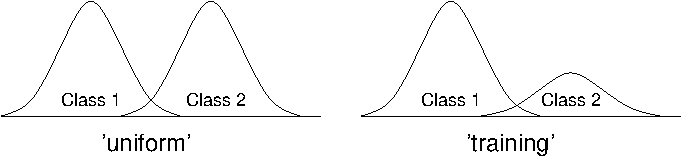
'uniform' (left) and 'training' (right) Regularize🔗
The parameter Regularize prevents the covariance matrix from collapsing, which can occur for linearly dependent data.
The default value of 0.0001 is recommended in most applications.
Evaluate the classifier🔗
The operator
can be used to evaluate the probabilities for a feature vector to belong to each of the available classes.
KSigmaProb🔗
The output parameter KSigmaProb describes the probability that another sample lies farther away from the mean of the corresponding class distribution.
Like the corresponding output of classify_class_gmm, KSigmaProb can be used for novelty detection. Feature vectors with a KSigmaProb below a selected threshold, for example 0.0001, can be rejected as novel samples.
Classify unknown samples🔗
Unknown feature vectors are classified with
Num🔗
The parameter Num specifies the number of best matching classes returned by the classifier.
In most applications, Num is set to 1.
A value greater than 1 can be useful if several possible classes are of interest, for example, when classes overlap.
KSigmaProb🔗
The output parameter KSigmaProb describes how well the feature vector fits the learned class distribution.
Like the corresponding output parameter of evaluate_class_gmm, it can be used for novelty detection.
All feature vectors with a KSigmaProb below a selected threshold, for example 0.0001, can be rejected as novel samples.
Novelty detection with GMM🔗
GMM classifiers can also be used for novelty detection.
For novelty detection, the classifier is trained using samples of a single class. During classification, feature vectors that significantly deviate from the learned class distribution can be rejected.
No additional novelty-detection mode is required. Instead, the novelty decision is based on the probability distribution learned from the training samples.
Classifier creation🔗
Novelty detection is realized by creating a classifier with a single class.
A GMM classifier is created with
Training samples can be added with
The classifier is trained with
Typical applications include
- defect detection,
- anomaly detection,
- change detection.
Classification🔗
Classification is performed with
Unknown samples are accepted if they fit the learned class distribution. Samples that significantly deviate from this distribution are rejected as novel samples.
The output parameter KSigmaProb can be used to determine whether a sample fits the trained class distribution.
The following example demonstrates novelty detection using a GMM classifier:
* Create a one-class GMM classifier
create_class_gmm (5, 1, [1,5], 'spherical', 'normalization', 5, 42, GMMHandle)
* Add training samples
for I := 0 to |Features|-1 by 1
    add_sample_class_gmm (GMMHandle, Features[I], 0, 0)
endfor
* Train the classifier
train_class_gmm (GMMHandle, 100, 0.001, 'equal', 0.0001, Centers, Iter)
* Classify unknown samples
classify_class_gmm (GMMHandle, FeatureVector, 1, ClassID, ClassProb, Density, KSigmaProb)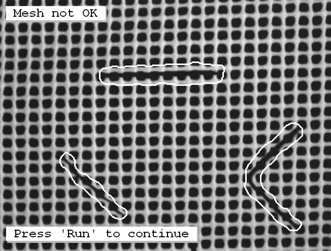
Parameter setting for GMM (Segmentation)🔗
Most considerations for parameter optimization are identical to those for general GMM classification.
For image segmentation, feature vectors are implicitly defined by the selected image channels. Therefore, no explicit feature extraction is required. The quality of the selected training regions has a significant influence on the classification result.
Adding samples🔗
Training regions are added using
The parameter Randomize behaves analogously to general GMM classification and is mainly used to compensate for undesired effects caused by integer-valued features.
Representative training regions are essential for obtaining robust segmentation results. The selected regions should
- cover the expected variations within a class,
- avoid ambiguous boundaries,
- contain sufficient samples for each class.
Training🔗
Training is performed with
The same considerations regarding MaxIter, Threshold, ClassPriors, and Regularize apply as for general GMM classification.
Classification🔗
Segmentation is performed with
Each pixel is assigned to the most probable class according to its feature vector.
The classification quality strongly depends on
- the selected image channels,
- the quality of the training regions,
- the representativeness of the training samples.
Practical recommendations🔗
For segmentation applications, it is recommended to
- select homogeneous training regions,
- avoid mixed pixels near class boundaries,
- use representative training images,
- optimize the selected image channels,
- verify the segmentation result visually.
If the classes overlap significantly, additional image channels or preprocessing steps should be considered.
Optimize critical parameters with a test application🔗
The classification performance strongly depends on the selected parameters and the quality of the training data. Therefore, critical parameters should not be optimized using only the training data.
To estimate the generalization ability of the classifier and to avoid overfitting, critical parameters should be optimized using independent test data. Cross validation provides an effective method for estimating the expected classification performance on previously unseen data.
Cross validation🔗
Cross validation divides the available training data into several subsets.
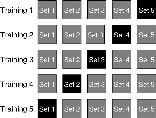
Typically, five subsets are used. During each iteration, one subset is used for testing while the remaining subsets are used for training. The procedure is repeated until every subset has been used once as the test set.
The average classification rate over all iterations provides an estimate of the expected classification performance on previously unseen data.
Cross validation is especially useful if
- only limited training data is available,
- different parameter settings are compared,
- overfitting is suspected,
- different feature combinations are evaluated.
Parameter optimization🔗
Critical parameters should be optimized one after another while keeping the remaining parameters unchanged.
Typical parameters include
NumCenters,CovarType,ClassPriors,Randomize,- the selected features.
For each parameter configuration:
- Train the classifier.
- Evaluate the classification result.
- Compare the obtained performance.
- Select the parameter configuration with the best generalization performance.
Parameter optimization should always be performed using independent test data or cross validation.
Representative datasets🔗
The quality of the classifier strongly depends on the representativeness of the training and test data.
The datasets should
- cover the expected variations,
- contain sufficient samples for every class,
- represent the expected application conditions.
If the class frequencies in the training data do not correspond to the expected occurrence frequencies during operation, the parameter ClassPriors should be adjusted accordingly.
Avoid overfitting🔗
A classifier that performs well on the training data does not necessarily generalize well to previously unseen samples.
Typical indications of overfitting include
- very high training accuracy,
- poor test accuracy,
- strong sensitivity to noise,
- unstable classification results.
Using unnecessarily many Gaussian centers or an overly flexible covariance model can increase the complexity of the classifier.
Cross validation and independent test datasets help to detect such effects.
Runtime optimization🔗
Only after satisfactory classification quality has been achieved should the runtime be optimized.
Possible measures include
- reducing the number of Gaussian centers,
- selecting a simpler covariance type,
- reducing the feature dimension using
Preprocessing, - reducing
NumComponentswhere appropriate, - reducing
MaxIterif the classification quality remains sufficient.
The covariance type provides an important trade-off between model flexibility and computational complexity. The complexity increases from 'spherical' over 'diag' to 'full'.
Runtime optimization should only be performed after the classification quality has been validated.
OCR classification with GMM features🔗
OCR operators can also be used to classify general objects if these objects can be described sufficiently by the available OCR features.
Compared to general feature classification, explicit feature extraction is not required because the OCR operators automatically extract the required features. This simplifies the workflow and may improve the runtime.
Since many OCR features are not rotation invariant, the objects should be aligned before training and classification.
Typical applications include
- classification of printed parts,
- classification of symbols,
- classification of simple geometric objects,
- character recognition.
Advantages of OCR operators🔗
OCR operators provide
- automatic feature extraction,
- optimized classification routines,
- efficient handling of large training sets,
- support for different classifier types.
In many applications, OCR classification can replace manually selected feature vectors.
Create an OCR classifier🔗
Depending on the desired classifier type, one of the following operators can be used:
During classifier creation, specify the character size and the class names.
WidthCharacter := 8
HeightCharacter := 10
Classes := ['good','bad']
create_ocr_class_mlp (8, 10, 'constant', 'default', Classes, 80, 'none', 10, 42, OCRHandle)
Define training data🔗
Representative training samples are essential for obtaining robust classification results.
The training objects should
- have similar dimensions,
- be aligned consistently,
- cover the expected variations,
- contain sufficient samples for each class.
Create a training file🔗
Training samples are stored using
The resulting training file can subsequently be reused for training different OCR classifier types.
write_ocr_trainf (Character, 'good', TrainingFile)
append_ocr_trainf (Character, 'bad', TrainingFile)
Train the classifier🔗
Training is performed with
During training, the OCR features are extracted automatically.
trainf_ocr_class_mlp (TrainingFile, 200, 1, 0.01, OCRHandle, Error, ErrorLog)Classification🔗
Objects are classified using
The operators return
- the predicted class,
- the corresponding confidence,
- additional classification information.
do_ocr_single_class_mlp (Character, OCRHandle, 1, Class, Confidence)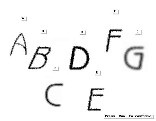
Practical recommendations🔗
For robust OCR classification, it is recommended to
- align the objects before classification,
- use representative training samples,
- avoid large scale variations,
- ensure good image quality,
- validate the classifier using independent test images.
If the objects exhibit large rotations or deformations, general feature classification or deep learning approaches may be more suitable.
Visualize the feature space (2D and 3D)🔗
Visualizing the feature space helps to understand the distribution of the training samples and to assess the separation between classes. It is particularly useful during feature selection, parameter optimization, and the analysis of classification errors.
Visualize the 2D feature space🔗
For two-dimensional feature vectors, the feature space can be displayed directly. The following example extends the citrus-fruit classification workflow and illustrates how the selected features separate the classes.
The feature vectors are constructed from the features
- area,
- circularity.
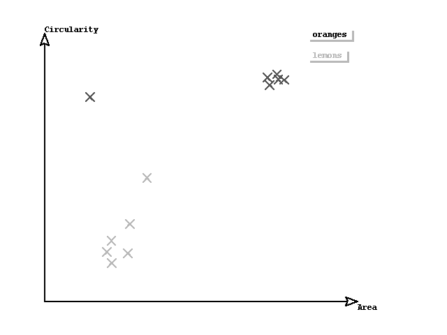
Well-separated clusters indicate that the selected features are suitable for classification. If significant overlaps occur, additional or different features should be considered.
Scaling🔗
Before plotting, the feature values are mapped to image coordinates.
ExtentOfGraph := Height - 0.3 * Height
RangeC := 0.5
RangeA := 24000
ScaleC := ExtentOfGraph / RangeC
ScaleA := ExtentOfGraph / RangeATranslation🔗
The minimum feature values are used to shift the coordinate system.
MinC := 0.5
MinA := 20000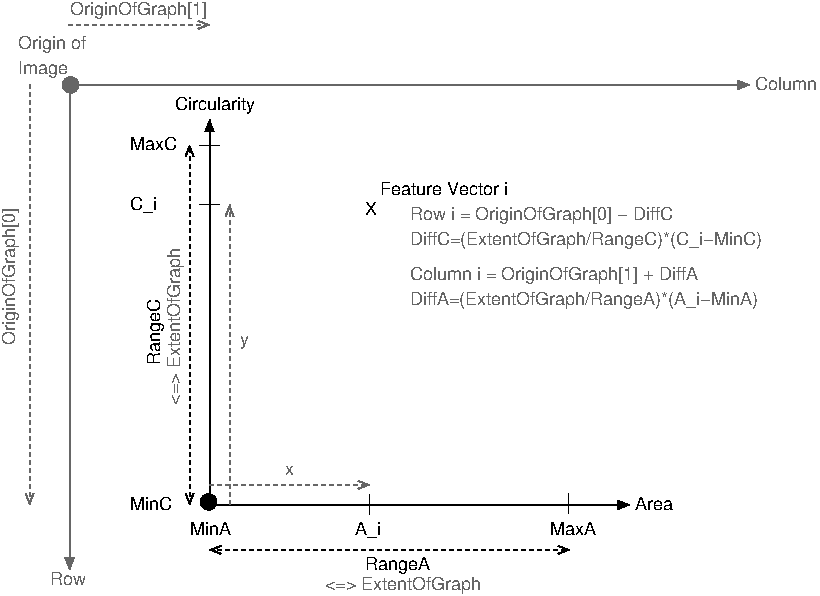
Plotting points🔗
Finally, the feature vectors are displayed as crosses.
for I := 0 to NumberFeatureVectors - 1 by 1
    DiffC := ScaleC * (FeaturesC[I] - MinC)
    DiffA := ScaleA * (FeaturesA[I] - MinA)
    RowFeature := OriginOfGraph[0] - DiffC
    ColumnFeature := OriginOfGraph[1] + DiffA
    gen_cross_contour_xld (Cross, RowFeature, ColumnFeature, CrossSize, 0.785398)
    dev_display (Cross)
endfor
Visualize the 3D feature space🔗
For three-dimensional feature vectors, feature-space visualization provides additional insight into the class distribution. It can help to identify compact clusters, overlapping regions, outliers, and class boundaries.
Typical applications include
- texture classification,
- surface inspection,
- material classification.
Transformations🔗
To display the feature vectors, geometric transformations are applied. Typical operators include
The transformations allow the feature space to be rotated and projected into the image plane.
hom_mat3d_translate (HomMat3DIdentity, Tx, Ty, Tz, HomMat3DTranslate)
hom_mat3d_scale (HomMat3DTranslate, Scale, Scale, Scale, 0, 0, 0, HomMat3DScale)
hom_mat3d_rotate (HomMat3DScale, Phi, 'x', 0, 0, 0, HomMat3DRotate)
project_3d_point (HomMat3DRotate, X, Y, Z, Row, Column)
Practical recommendations🔗
Feature-space visualization is recommended during feature engineering, parameter optimization, and the analysis of classification results. It helps to assess the discriminative power of the selected features and to detect outliers or overlapping classes.
If significant overlaps occur between classes, additional features or a different classification method should be considered.