Handling images in HALCON🔗
In HALCON terminology, images are iconic data.
The other iconic parameter types are regions and XLD data.
For more information, see Parameters and data structures on the HALCON architecture and general concepts page.
To understand the different types of images you can process in HALCON, the three components of an image are explained in the following sections: pixels, channels, and domains.
Tip
To learn more about the basic concept of images in HALCON, take a look at the HDevelop example program halcon_basic_concepts.hdev.
About pixels🔗
In HALCON, pixels can be used to represent information of various kinds. Therefore, different pixel types are distinguished.
Table 1 lists the different pixel types and the corresponding standard image types for images.
Note that this list is not exclusive (for example, a gray value image can belong to multiple other image types as well).
You can convert the image type using convert_image_type.
| Pixel type | Standard image type |
|---|---|
| Gray values | byte, uint2 |
| Difference | int1, int2 |
| 2D histogram | int4 |
| Edge directions | direction |
| Derivatives | real |
| Fourier transform | complex |
| Hue values | cyclic |
| Vector field | vector_field1 |
There is also the image type int8 (64 bits with sign), which is only available on 64 bit systems
Gray values🔗
Gray images are of type byte (8 bits without sign) or uint2 (16 bits without sign) and consist of pixels usually representing local intensities of light on a sensor.
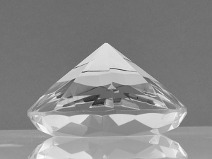
Figure 1. Gray value image
Difference🔗
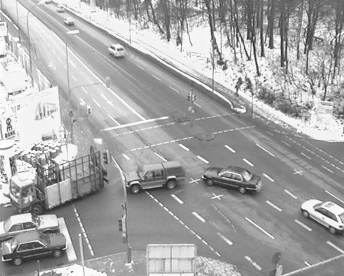
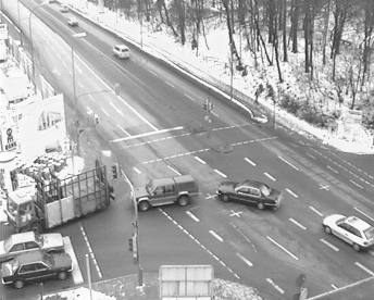
To show the differences between two images, for example, the image types int1 (8 bits with sign) or int2 (16 bits with sign) are well suited.
 |
 |
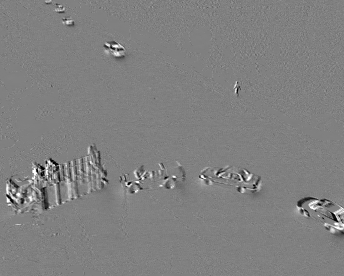 |
Figure 2. Comparing an image with another (for example, consecutively taken) one by subtracting the latter from the former results in a difference image .
2D histogram🔗
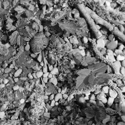
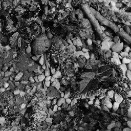
To examine image features based on the occurrence of gray values in two images, you can use a 2D histogram, which is of type int4 (32 bits with sign).
The axes of the 2D histogram each represent the gray values of an input image.
The gray values of corresponding pixels in the input images are registered in the 2D histogram accordingly.
The higher the frequency of a specific combination of gray values, the higher the gray value in the output image (see also histo_2dim).
 |
 |
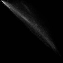 |
Figure 3.
,
Two channels of an exemplary image
Their 2D histogram
Edge directions🔗
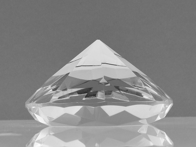
To represent the orientation of the edge gradient, the image type direction (8 bits without sign) is available.
 |
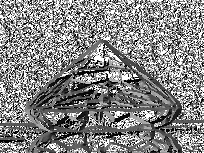 |
Figure 4. Examining an image by visualizing the orientation of its image edges
For images of type direction, an edge direction of \(x\) degrees in mathematically positive sense and with respect to the horizontal axis is stored as \(x / 2\) in the edge direction image (resulting in gray values from 0 to 179).
Points with edge amplitude 0 are assigned the edge direction 255 (undefined direction).
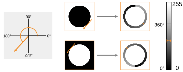
Figure 5. Visualizing the edge directions for dark and bright objects using sobel_dir.
The edge direction (marked with an tangential arrow in the input image) of a pixel is encoded by a corresponding gray value in the result image on the right.
Locations without an edge are represented by a gray value of 255.
Derivatives🔗
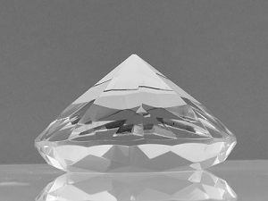
The image type real (32 bits floating point value) is used to represent derivatives of an image, for example, to extract edges.
 |
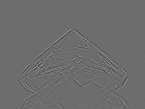 |
Figure 6. Some features of an image (for example, edges, gradients) can be examined by considering its derivatives .
Fourier transform🔗
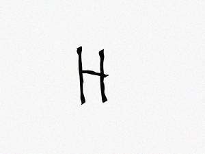
To inspect the frequency domain of an image, the Fourier transform is used.
The combination of magnitude and phase of the frequencies is represented by complex numbers.
Therefore, the image type is complex (two real values per pixel).
 |
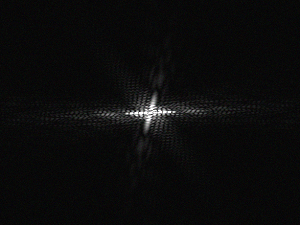 |
Figure 7. One strategy to identify letters is to observe its frequency domain by calculating the Fourier transform .
Hue values🔗
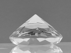
Hue values are encoded cyclic (8 bits without sign), such that \(255+1 = 0\).
 |
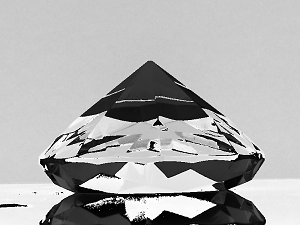 |
Figure 8. Pixels representing hue values
When increasing a pixel value beyond 255, it is shifted to the other end of the spectrum.
Adding a constant number to each cyclic pixel value of
results in an image like
.
Vector field🔗
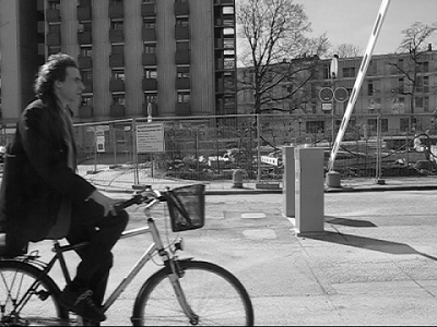
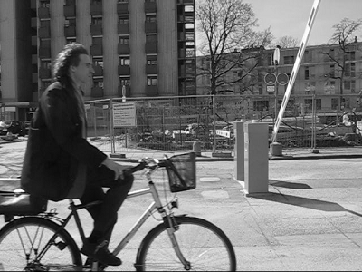
A special image type to represent absolute/relative optical flow is vector_field (composed by two real images for x and y direction).
The type of vector field can be specified further by assigning vector_field_absolute (interpreted as absolute coordinates) or vector_field_relative (interpreted as vectors).
 |
 |
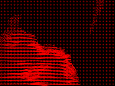 |
Figure 9. Relative motion of pixels (for example, in consecutive images and ) can be represented in a vector field .
About channels🔗
Besides different pixel types, an image can use different image channels to store specific information. Basically, you can use channels to assign multiple values to a pixel. The following sections mention a few cases, where different numbers of channels are useful.
Gray value images (single-channel images)🔗
Often, there is only one value stored for every pixel of an image. A gray value image, for example, stores a value representing local light intensity on a sensor for each pixel.
Nevertheless, various types of information can be assigned to those pixels (for example, the derivatives of gray values, distances). Visualizing them analogous to a gray value image can help interpreting the data.
RGB images (three-channel images)🔗
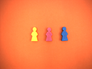
For a colored image, the pixel values are typically stored in three channels, each representing the intensity of either red, green, or blue light of the respective pixel (RGB image). Through additive mixing of the three values assigned to one pixel, a specific color is defined.
Apart from the RGB model there are several further color spaces.
For more information about those models and how to transform between the different color spaces, see trans_to_rgb and trans_from_rgb, respectively.
 |
 |
 |
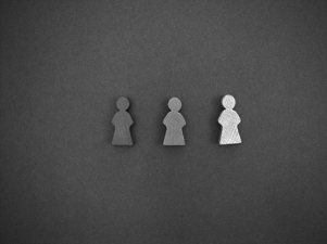 |
Figure 10.
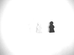
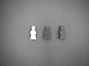
RGB image and its three separate channels:
The local intensities differ for the red
, green
, and blue channel
.
Multispectral images (multi-channel images)🔗
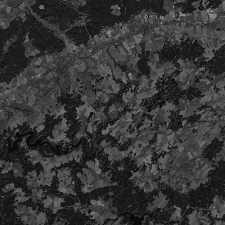
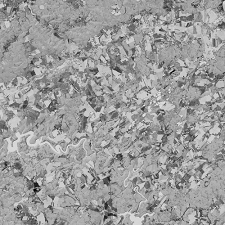
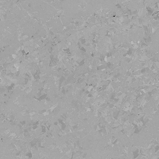
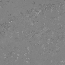
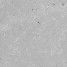
Special cameras can register a variety of spectral bands in an image, including those outside the visible light spectrum. Satellite cameras, for instance, often acquire multispectral data and store them in corresponding multiple distinct channels.
 |
 |
 |
 |
 |
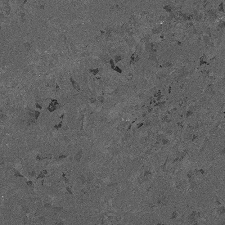 |
Figure 11. Six channels of an satellite image
The different channels of a multispectral image can be used to extract features that are most prominent in a special spectral band.
Multi-channel images🔗
Besides representing light intensities, assembling multiple channels in one image can help with various other tasks.
For example, combining a gray value image with an additional channel containing the respective depth values of the image pixels allows you to visualize the scene in a 3D plot.
Instead of using a depth camera you can also use a multi-channel image to extract depth information. Therefore, each channel must contain one of a series of images taken with different focus levels.
Besides containing spacial information, the channels of an image can also be interpreted as a feature space to perform a principal components analysis.
About domains🔗
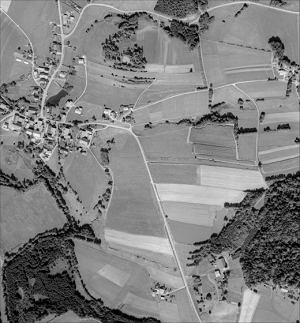
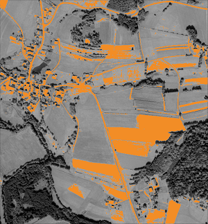
The image domain determines the area of an image that is used in the succeeding operations. You can reduce the domain to the relevant parts of an image to focus the processing on regions of interest or speed up the operations.
 |
 |
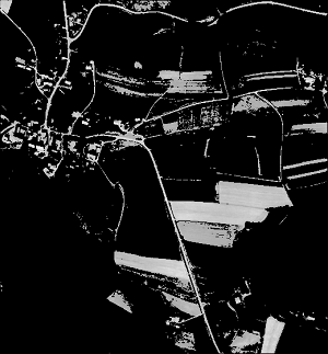 |
Figure 12.
Original image
The domain of the image is reduced, for example, considering a minimum gray value threshold .
In the resulting image, areas that are still relevant for further operations (orange) remain, whereas unwanted areas of the image are excluded (black).
-
The image type
vector_fieldcan be specified further by usingvector_field_absoluteorvector_field_relative. ↩