About deep learning with HALCON🔗
More Info
Get an introduction to deep learning or learn about datasets for deep learning and many other topics in interactive online courses at our MVTec Academy.
Available methods🔗
The term deep learning (DL) refers to a family of machine learning methods. In HALCON, the following methods are implemented:
- 3D Gripping Point Detection
-
Detect gripping points on objects in a 3D scene. For more information, see 3D Matching > 3D Gripping Point Detection.
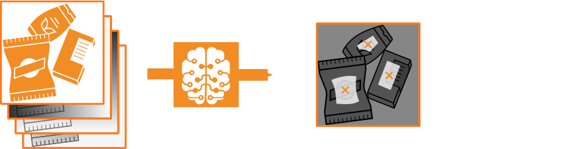
Figure 1. A possible example for a 3D Gripping Point Detection application: A 3D scene (for example, an RGB image and XYZ-images) is analyzed and possible gripping points are suggested.
- Advanced object detection
-
Detect objects of the given classes and localize them within the image. For more information, see Advanced object detection.


Figure 2. A possible example for advanced object detection: Within the input image three instances are found and assigned to a class.
- Anomaly detection and Global Context Anomaly Detection
-
Assign to each pixel the likelihood that it shows an unknown feature. For more information, see Anomaly detection.
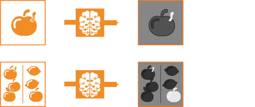
Figure 3. Top: A possible example for anomaly detection: A score is assigned to every pixel of the input image, indicating how likely it shows an unknown feature, i.e., an anomaly. Bottom: A possible example for Global Context Anomaly Detection: A score is assigned to every pixel of the input image, indicating how likely it shows a structural or logical anomaly.
- Classification
-
Classify an image into one class out of a given set of classes. For more information, see Classification.


Figure 4. A possible example for classification: The image gets assigned to a class.


Figure 5. A possible example for Out-of-Distribution Detection for classification: The image is assigned to a class and identified as Out-of-Distribution, if applicable.
- Continual Learning
-
Extend a classification model with new data to learn additional classes or to improve the performance on existing classes. For more information, see Continual Learning.
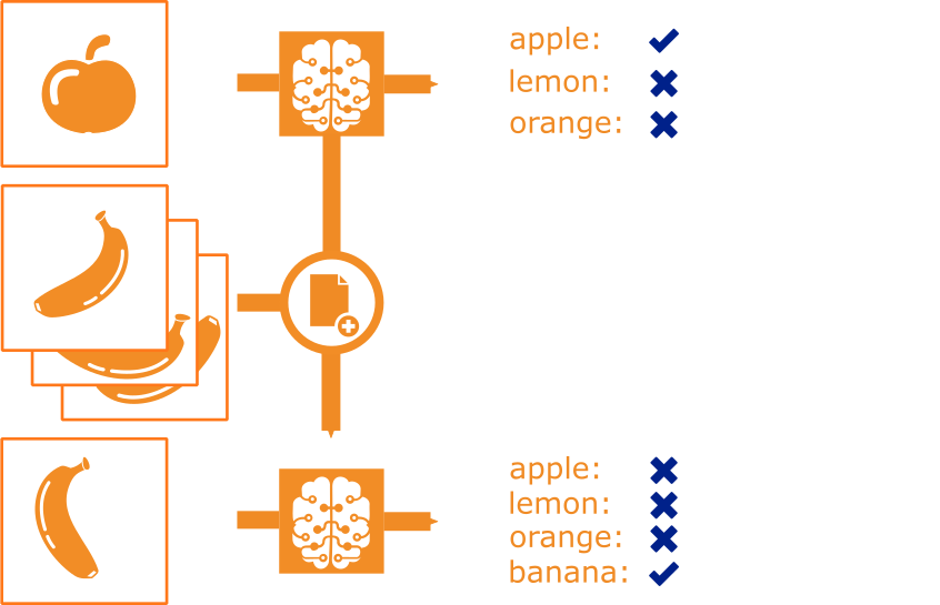
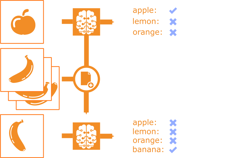
Figure 6. A possible example for Continual Learning: A classification model is extended with a new class.
- Deep 3D Matching
-
Detect objects in a scene and compute their 3D pose. For more information, see Deep 3D Matching.
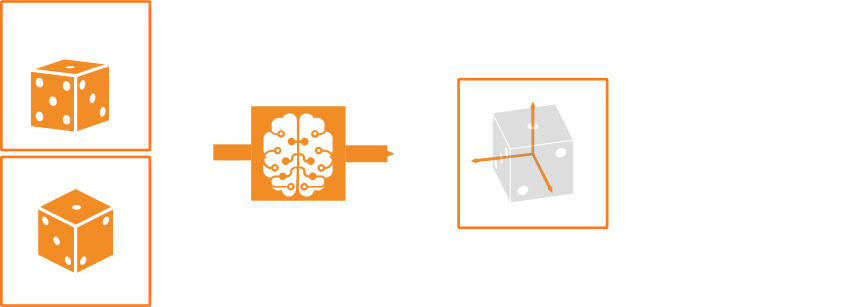
Figure 7. A possible example for a Deep 3D Matching application: Images from different angles are used to detect an object. As a result, the 3D pose of the object is computed.
- Deep Counting
-
Detect and count objects in images. For more information, see Deep Counting.


Figure 8. A possible example for a Deep Counting application: Objects in an image are counted and the object quantity is returned.
- Deep OCR
-
Detect and recognize words (not just characters) in an image. For more information, see OCR > Deep OCR.


Figure 9. A possible example for deep-learning-based optical character recognition: Words in an image are detected and recognized.
- Instance segmentation and object detection
-
Detect objects of the given classes and localize them within the image. Instance segmentation is a special case of object detection, where the model also predicts distinguished object instances and additionally assigns for the found instances their region within the image. For more information, see Instance segmentation and object detection.


Figure 10. A possible example for instance segmentation: Every instance gets its individual region marked.
Figure 11. A possible example for object detection: Within the input image three instances are found and assigned to a class.
- Multi-label classification
-
An image is assigned all contained classes from a given set of classes. For more information, see Multi-label classification.


Figure 12. A possible example for multi-label classification: All contained classes are assigned to the image.
- Semantic segmentation and edge extraction
-
Assign a class to each pixel of an image, but different instances of a class are not distinguished. A special case of semantic segmentation, where every pixel of the input image is assigned to one of the two classes “edge” and “background”. For more information, see Semantic segmentation and edge extraction.
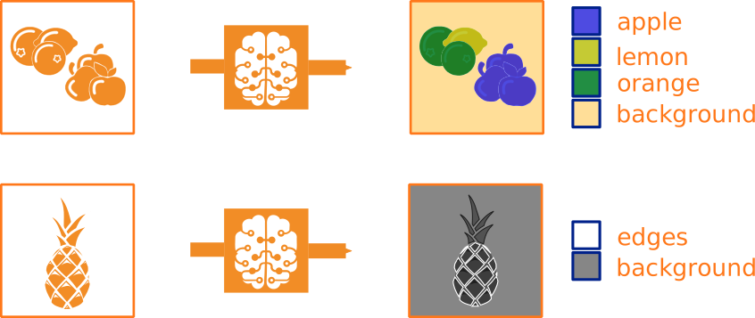
Figure 13. Top: A possible example for semantic segmentation: Every pixel of the input image is assigned to a class. Bottom: A possible example for edge extraction: Pixels belonging to specific edges are assigned to the class “edge”.
All of the deep learning methods listed above use a network for the assignment task. In HALCON, they are implemented within the general DL model; see HALCON DL model.
The model is trained by only considering the input and output, which is also called end-to-end learning.
In essence, the training algorithm uses images and the information visible in them to adjust the model to distinguish different classes and, eventually, find the corresponding objects.
As a user, you do not need to specify the features manually.
Instead, you have to select and collect appropriate data.
System requirements and license information🔗
For deep learning, additional prerequisites apply. For more information, see the requirements listed in Requirements for deep learning and deep-learning-based methods.
The required module license depends on the model type used in your application. For more information, see Dynamic modules for deep-learning-based applications.
About the general workflow🔗
As the DL methods mentioned above differ in what they do and how they need the data, you need to know which method is most appropriate for your specific task. Once this is clear, you need to collect a suitable amount of data, that is, images and the information needed by the method. After that, there is a common general workflow for all these DL methods:
-
Prepare the network and the data.
The network needs to be prepared for your task and your data adapted to the specific network.
-
Get a network: Read in a pretrained network or create one.
-
The network needs to know which problem it shall solve, i.e., which classes are to be distinguished and what such samples look like. This is represented by your dataset, i.e., your images with the corresponding ground truth information.
-
The network will impose several requirements on the images (as, for example, the image dimension, gray value range, … ). Therefore, the images have to be preprocessed so that the network can process them.
-
We recommend splitting the dataset into three distinct datasets used for training, validation, and testing.
-
-
Train the network and evaluate the training progress.
Once your network is set up and your data prepared, train the network for your specific task.
-
Set the hyperparameters appropriate to your task and system.
-
Optionally, specify your data augmentation.
-
Start the training and evaluate your network.
-
-
Apply and evaluate the final network.
Your network is trained for your task and ready to be applied. However, you should evaluate how well the network performs on basis of your test dataset before deploying it in the real world.
-
Start the inference phase.
When your network is trained and you are satisfied with its performance, you can use it for inference on new images. For this, the images need to be preprocessed according to the requirements of the network (this means, in the same way as for the training).
About data🔗
In the context of deep learning, the term “data” refers to images and the information they contain. The latter information has to be provided in a way the network can understand.
About data requirements🔗
Evidently, the different DL methods have their own requirements concerning what information has to be provided and how. See the corresponding chapters for the specific requirements.
The network further poses requirements on the images regarding the image dimensions, the gray value range, and the type.
The specific values depend on the network and can be queried with get_dl_model_param.
Additionally, depending on the method there are also requirements regarding the information as, for example, the bounding boxes.
To fulfill all these requirements, the data may have to be preprocessed, which can be done most conveniently with the corresponding procedure preprocess_dl_samples.
To train the network, use representative images, that is, images like the ones you want to process later and not only “perfect” images. Otherwise, the network may have difficulties with non-“perfect” images.
About data splitting🔗
When you train your network, the network gets adapted to its task.
At one point, you will want to evaluate what the network learned and later, you will want to test the network.
Therefore, the dataset is split into three subsets, which should be independent and identically distributed.
In simple words, the subsets should not be connected to each other in any way and each set should contain the same distribution of images for every class.
This splitting can conveniently be done by the procedure split_dl_dataset.
The largest subset will be used for the retraining.
We refer to this dataset as the training dataset.
At a certain point, the performance of the network is evaluated to check whether it is beneficial to continue the network optimization.
For this validation, the second set of data is used: the validation dataset.
Even if the validation dataset is disjoint from the first one, it has an influence on the network optimization.
Therefore, to test the possible predictions when the model is deployed in the real world, the third dataset is used: the test dataset.
For a representative network validation or evaluation, the validation and test datasets should contain statistically relevant data, which gives a lower bound on the amount of needed data.
About the network and the training process🔗
In the context of deep learning, the assignments are performed by sending the input image through a network. The output of the total network consists of a number of predictions. For a classification task, for example, such a prediction is the confidence for each class, expressing how likely the image shows an instance of this class.
The specific network will vary, especially from one method to another. Some methods like object detection use a subnetwork to generate feature maps (see the explanations given below and in Object detection and instance segmentation).
Here, we will explain a basic Convolutional Neural Network (CNN). Such a network consists of a certain number of layers or filters, which are arranged and connected in a specific way. In general, any layer is a building block performing specific tasks. It can be seen as a container, which receives input, transforms it according to a function, and returns the output to the next layer. Thereby, different functions are possible for different types of layers.
More Info
TODO: Several possible examples are given in the “Solution Guide on Classification".
Many layers or filters have weights parameters, which are also called filter weights.
These are the parameters modified during the training of a network.
The output of most layers are feature maps.
The number of feature maps (the depth of the layer output) and their size (width and height) depend on the specific layer.
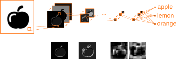
Figure 14. Schema of an extract of a possible classification network. Below: Feature maps corresponding to the layers, zoomed to a uniform size
To train a network for a specific task, a loss function is added. There are different loss functions depending on the task, but they all work according to the following principle:
A loss function compares the prediction from the network with the given information, what to find in the image (and, if applicable, also where), and penalizes deviations.
Now, the filter weights are updated in such a way that the loss function is minimized.
Thus, when training the network for the specific tasks, one strives to minimize the loss (an error function) of the network, assuming that this will also improve the performance measure.
In practice, this optimization is done by calculating the gradient and updating the parameters of the different layers (filter weights) accordingly.
This is repeated by iterating multiple times over the training data.
There are additional parameters that influence the training, but which are not directly learned during the regular training. These parameters have values set before starting the training. We refer to this last type of parameters as hyperparameters to distinguish them from the network parameters that are optimized during training. For more information, see Setting the training parameters: hyperparameters below.
To train all filter weights from scratch, a lot of resources are needed.
Therefore, one can take advantage from the following observation:
The first layers detect low level features like edges and curves.
The feature map of the following layers are smaller, but they represent more complex features.
For a large network, the low level features are general enough so the weights of the corresponding layers will not change much among different tasks.
This leads to a technique called transfer learning:
Take an already trained network and retrain it for a specific task, benefiting from already quite suitable filter weights for the lower layers.
As a result, considerably less resources are needed.
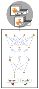
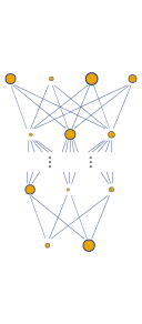
While in general the network should be more reliable when trained on a larger dataset, the amount of data needed for retraining also depends on the complexity of the task. A basic schema for the workflow of transfer learning is shown with the aid of classification in the figure below.
 |
 |
 |
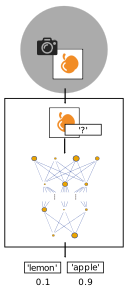 |
Figure 15. Basic schema of transfer learning with the aid of classification.
A pretrained network is read.
Training phase, the network gets trained with the training data.
The trained model with new capabilities.
Inference phase, the trained network infers on new images.
Setting the training parameters: hyperparameters🔗
The different DL methods are designed for different tasks and will vary in the way they are built up. They all have in common that the training of the model leads to a minimization problem. Training the network or subnetwork strives to minimize a corresponding loss function (see About the network and the training process). For doing so, there is a set of further parameters which is set before starting the training and not optimized during the training. We refer to these parameters as hyperparameters. For a DL model, you can set a change strategy, specifying when and how you want these hyperparameters changed during the training. Note that certain methods have additional hyperparameters. You find more information in their respective chapter.
As already mentioned, the loss compares the predictions from the network with the given information about the content of the image.
The loss penalizes deviations.
Training the network means updating the filter weights in such a way that the loss has to penalize less, thus the loss result is optimized.
To do so, a certain amount of data is taken from the training dataset.
For this subset, the gradient of the loss is calculated and the network is modified by updating its filter weights accordingly.
Now, this is repeated with the next subset of data untill the whole training data is processed.
These subsets of the training data are called batches and the size of these subsets, the batch size, determines the number of data taken into a batch, processed together.
A full iteration over the entire training data is called epoch.
It is beneficial to iterate several times over the training data.
The number of iterations is defined by 'epochs'.
Thus, 'epochs' determines how many times the algorithm loops over the training set.
Some models (for example, anomaly detection) train utilizing the whole dataset at once. For other models, the dataset is processed batch-wise and in order to do so, the SGD (stochastic gradient descent algorithm) or Adam (adaptive moment estimation) can be used. This involves further parameters, which are explained in the following.
After every calculation of the loss gradient the filter weights are updated. For this update, there are two important hyperparameters:
'learning_rate'λ, determining the weight of the gradient on the updated loss function arguments (the filter weights)'momentum'μ within the interval \([0,1)\), specifying the influence of previous updates.
For more information, see train_dl_model_batch.
In simple words, when we update the loss function arguments, we still remember the step we took for the last update.
Now, we take a step in direction of the gradient with a length depending to the learning rate.
Additionally, we repeat the step we did last time, but this time only μ times as long.
A visualization is given in the figure below.
A too large learning rate might result in divergence of the algorithm; a very small learning rate will take unnecessarily many steps.
Therefore, starting with a larger learning rate and potentially reduce it during training is recommended.
With μ = 0, the momentum method has no influence, and only the gradient determines the update vector.
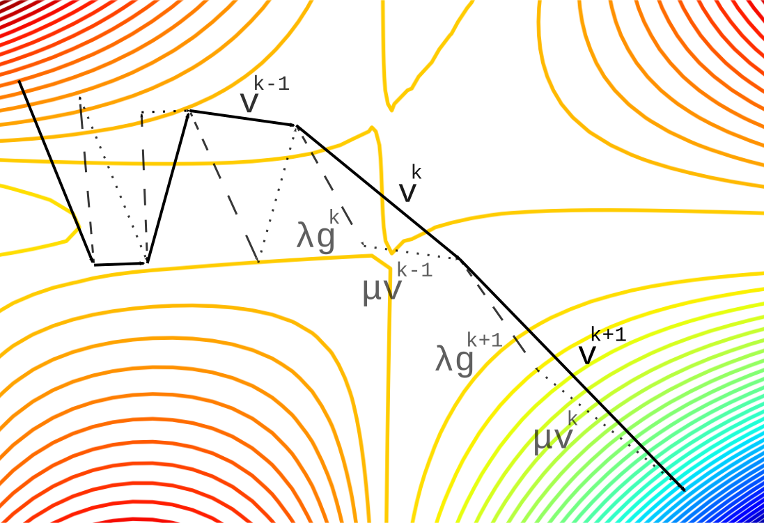
Figure 16. Sketch of the 'learning_rate' and the 'momentum' during an actualization step.
The gradient step: the learning rate λ times the gradient g (λg – dashed lines).
The momentum step: the momentum μ times the previous update vector v (μv – dotted lines).
Together, they form the actual step: the update vector v (v – solid lines).
To prevent the neural networks from overfitting (see Risk of underfitting and overfitting below), regularization can be used.
Simply put, regularization favors simpler models that are less likely to fit to noise in the training data and generalize better.
In HALCON, the model weights can be regularized using L2 regularization or weight decay:
- L2 regularization works by adding an extra term to the loss function, which penalizes the squared magnitude of the weights.
- Weight decay directly shrinks the magnitude of the weights by a small factor in each iteration of the training.
L2 regularization and weight decay have the same effect in the SGD solver.
Therefore, we recommend using only one of the two methods at a time.
For the Adam solver, weight decay should be preferred over L2 regularization.
For more information, see train_dl_model_batch.
The weight regularization can be controlled by the hyperparameters 'weight_prior' and 'weight_decay', respectively.
Choosing their value is a trade-off between the model’s ability to generalize, overfitting, and underfitting.
If the parameter value is too small, the model might overfit.
If it is too large, the model might lose its ability to fit the data well because all weights are pushed too close to zero.
With the training data and all the hyperparameters, there are many different aspects that can have an influence on the outcome of such complex algorithms. To improve the performance of a network, generally the addition of training data also helps. Whether to gather more data is a good solution always depends on how easily one can do so. Usually, a small additional fraction will not noticeably change the total performance.
Supervising the training🔗
The different DL methods have different results. Accordingly, they also use different measures to determine how well a network performs. When training a network, there are behaviors and pitfalls applying to different models, which are described below.
Validation during training🔗
When validating the network performance, this is not a pure optimization problem (see About the network and the training process and Setting the training parameters: hyperparameters above).
To observe the training progress, it is usually helpful to visualize a validation measure. For example, for the training of a classification network, this can be the error over the samples of a batch. As the samples differ, the difficulty of the assignment task may differ. Thus it can be that the network performs better or worse for the samples of a given batch than for the samples of another batch. It is hence normal that the validation measure is not changing smoothly over the iterations. However, in total it should improve.
Adjusting the hyperparameters 'learning_rate' and 'momentum' can help to improve the validation measure again.
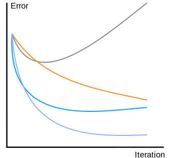
The following figures show possible scenarios.
  |
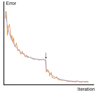 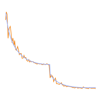 |
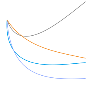
Figure 17. Validation measure during training, here using the error from classification as example.
General tendencies for possible outcomes with different 'learning_rate' values; purple: good learning rate, gray: very high learning rate, blue: high learning rate, orange: low learning rate.
Ideal case with a learning rate policy to reduce the 'learning_rate' value after a given number of iterations; orange: training error, purple: validation error.
The arrow marks the iteration at which the learning rate is decreased.
Risk of underfitting and overfitting🔗
Underfitting occurs if the model is not able to capture the complexity of the task. It is directly reflected in the validation measure on the training set, which stays high.
Overfitting happens when the network starts to “memorize” training data instead of learning how to generalize.
This is shown by a validation measure on the training set, which stays good or even improves while the validation measure on the validation set decreases.
In such a case, regularization may help.
For more informatoin, see the explanations of the hyperparameters 'weight_prior' and 'weight_decay' in Setting the training parameters: hyperparameters.
Note that a similar phenomenon occurs when the model capacity is too high with respect to the data.
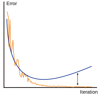
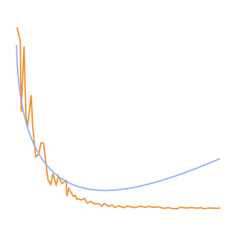
Figure 18. Possible overfitting scenario, visible on the generalization gap (indicated by the arrow). The error from classification serves as an example for a validation measure.
Confusion matrix🔗
For an instance, a network infers a top prediction, the class for which the network deduces the highest affinity. When we know its ground truth class, we can compare the two class affiliations: the predicted one and the correct one. The instance differs between the different types of methods. For example, in classification, the instances are images; in semantic segmentation, the instances are single pixels.
When more than two classes are distinguished, one can also reduce the comparison into binary problems. This means, for a given class you just compare if it is the same class (positive) or any other class (negative). For such binary classification problems, the comparison is reduced to the following four possible entities (not all are applicable for every method):
- True positives (TP: predicted positive, labeled positive)
- True negatives (TN: predicted negative, labeled negative)
- False positives (FP: predicted positive, labeled negative)
- False negatives (FN: predicted negative, labeled positive)
A confusion matrix is a table with such comparisons.
This table makes it easy to see how well the network performs for each class.
For each class, it lists how many instances have been predicted into which class.
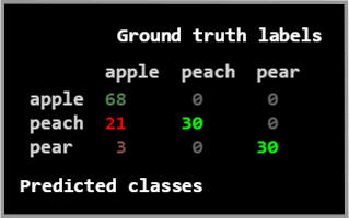
For example, for a classifier distinguishing the three classes “apple”, “peach”, and “orange”, the confusion matrix shows how many images with ground truth class affiliation “apple” have been classified as “apple” and how many have been classified as “peach” or “orange”.
This information is listed for the other classes as well.
An example is shown in the figure below.
In HALCON, for each class, we represent the instances with this ground truth label in a column and the instances predicted to belong to this class in a row.
 |
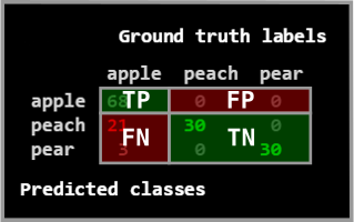 |
Figure 19. An example for a confusion matrices from classification.
68 images of an “apple” have been classified as such (TP), 60 images showing not an “apple” have been correctly classified as a “peach” (30) or “pear” (30, TN), 0 images show a “peach” or a “pear” but have been classified as an “apple” (FP), and 24 images of an “apple” have wrongly been classified as “peach” (21) or “pear” (3, FN).
A confusion matrix for all three distinguished classes.
It appears as if the network “confuses” apples and peaches more than all other combinations.
The confusion matrix of the binary problem to better visualize the “apple” class.
����