Multi-label classification🔗
Multi-label classification based on deep learning is a method, in which an image is assigned multiple confidence values. These confidence values indicate how likely the image belongs to each of the different classes. Thus, multi-label classification means to assign multiple specific classes to an image. This is illustrated in the following schema.
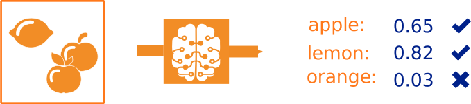
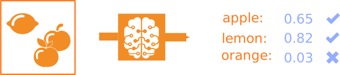
Figure 1. A possible multi-label classification example, in which the network has three classes. The input image is assigned confidence values for each of the three classes: “apple” 0.65, “lemon” 0.82, and “orange” 0.03. According to the top predictions, the image has the classes “apple” and “lemon”.
To classify your data into the classes you want to have distinguished, the classifier has to be trained accordingly.
HALCON uses a technique called transfer learning (see also the deep learning overview page).
Hence, we provide pretrained networks, representing classifiers that have been trained on huge amounts of labeled image data.
These classifiers have been trained and tested to perform well on industrial image classification tasks.
One of these classifiers, already trained for general classifications, is now retrained for your specific task.
For this, the classifier needs to know which classes are to be distinguished and how such examples look like.
This is represented by your dataset, i.e., your images with the corresponding ground truth labels.
For more information about the data requirements, see About data.
More Info
- In HALCON, multi-label classification with deep learning is implemented within the more general deep learning model. For more information about the latter, see Deep learning > HALCON DL model.
- For the specific system requirements to apply deep learning, see Requirements for deep learning and deep-learning-based methods.
About data🔗
We distinguish between data used for training and evaluation and data used for inference. While the latter consists of bare images, for the former you already know to which class the images belong and provide this information over the corresponding labels.
As a basic concept, the model handles data over dictionaries, meaning it receives the input data over a dictionary DLSample and returns the dictionaries DLResult and DLTrainResult.
For more information about data handling, see Deep learning > HALCON DL model.
- Data for training and evaluation
-
The dataset consists of images and corresponding information. They have to be provided in a way the model can process them. For more information about the image requirements, see Images.
The training data is used to train and evaluate a network for your specific task. With the aid of this data, the classifier can learn which classes are to be distinguished and how their representatives look like. In classification, the image is classified as a whole. Therefore, the training data consists of images and their ground truth labels, that is, the class you say this image belongs to.
Images should be as representative as possible for your task. How to store and retrieve this information is possible in different ways. For information about how to format the data, see Deep learning > HALCON DL model. In short, a dictionaryDLDatasetserves as a database for the information needed by the training and evaluation procedures.Although training a classifier using transfer learning needs less resources, you still need a suitable set of data. While in general the network should be more reliable when trained on a larger dataset, the amount of data needed for training also depends on the complexity of the task.
You also want enough training data to split it into three subsets: for training, for validation, and for testing the network. These subsets are preferably independent and identically distributed (see also About data splitting). - Images
-
Regardless of the application, the model poses requirements on the images, such as the dimensions, the gray value range, and the type. The specific values depend on the network itself and can be queried with
get_dl_model_param. For more information about specific values of different models, seeread_dl_model.To fulfill these requirements, you may have to preprocess your images. Standard preprocessing is implemented in the procedure
preprocess_dl_datasetand, for a sample, inpreprocess_dl_samples. In case of custom preprocessing, these procedures offer guidance on the implementation. - Model output
-
The network output depends on the task:
-
Training
As output, the operator will return a dictionary
DLTrainResultwith the current value of the total loss as well as values for all other losses included in your model. -
Inference and evaluation
As output, the network will return a dictionary
DLResultfor every sample. For each input image, this dictionary will include a tuple containing the confidence values for each class to be distinguished (in decreasing order), as well as a second tuple containing the corresponding class IDs.
-
Tip
If you have already a labeled multi-label classification dataset, you can use the procedure read_dl_dataset_multi_label_classification.
It formats the data and creates a dictionary DLDataset.
This procedure can also be used to create a DLDataset for multi-label classification from object detection, segmentation, or classification data.
Interpreting the multi-label classification results🔗
When classifying an image, we obtain a set of confidence values indicating the image’s affinity to each class. It is also possible to compute the following values.
- Precision
-
The precision is the proportion of all correct predicted positives to all predicted positives (true and false ones). Thus, it is a measure of how many positive predictions really belong to the selected class.
\[\begin{eqnarray*} \textrm{precision} = \frac{\textrm{TP}}{\textrm{TP} + \textrm{FP}} \end{eqnarray*}\] - Recall
-
The recall, also called the “true positive rate”, is the proportion of all correct predicted positives to all real positives. Thus, it is a measure of how many samples belonging to the selected class were predicted correctly as positives.
\[\begin{eqnarray*} \textrm{recall} = \frac{\textrm{TP}}{\textrm{TP} + \textrm{FN}} \end{eqnarray*}\]A classifier with high recall but low precision finds most members of positives (thus members of the class), but at the cost of also classifying many negatives as member of the class.
A classifier with high precision but low recall is just the opposite, classifying only few samples as positives, but most of these predictions are correct.
An ideal classifier with high precision and high recall will classify many samples as positive with a high accuracy. - F-score
-
To represent the above with a single number, we compute the F1-score, the harmonic mean of precision and recall. Thus, it is a measure of the classifier’s accuracy.
\[\begin{eqnarray*} \textrm{F1-score} = 2 \times \frac{\textrm{precision} \times \textrm{recall}}{\textrm{precision} + \textrm{recall}} \end{eqnarray*}\] - Mean average precision
-
The average precision (AP) value is the average of maximum precision at different recall values. In simple words, it tells whether the classes predicted for the images are generally correct predictions or not. In this context, we pay more attention to the predictions with high confidence values. The higher the value, the better.
You can obtain the specific AP values: the averages over the classes, the averages over the thresholds, and the averages over both the classes and the thresholds. The latter is the mean average precision (mAP), a measure of how well images are classified.