Gray value interpolation🔗
Gray value interpolation interpolates between the gray values of more than one pixel of an
original image.
It is a method that is necessary for image transformations.
If an image is rotated and downscaled, a resulting pixel of the output image does not correspond to exactly one pixel of
the input image anymore.
Instead, it may contain parts of more than one pixel of the original image.
Therefore, a method to calculate the gray value of the resulting pixel is required.
Interpolation methods🔗
Nearest neighbor interpolation (‘nearest_neighbor’)🔗
If ‘nearest_neighbor’ is selected, no interpolation over multiple pixels is performed.
Instead, the resulting pixel is assigned the gray value of the pixel in the original image whose center lies closest to the center of the resulting
pixel.
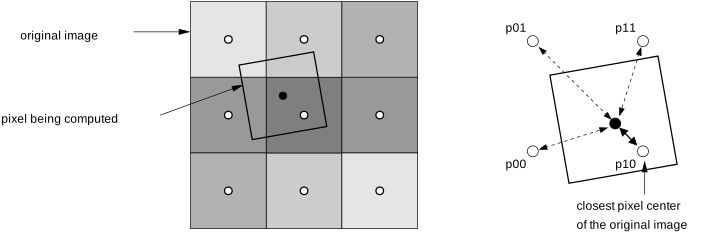
The resulting pixel receives the gray value of pixel p10.
Nearest neighbor interpolation is the simplest and fastest approach for determining the gray value of the resulting pixel. But typically, it leads to undesired effects like aliasing and jagged edges if the image is rotated or scaled.
Bilinear interpolation (‘bilinear’)🔗
If ‘bilinear’ is selected, the gray values are determined using bilinear interpolation. In contrast to nearest neighbor interpolation, in bilinear interpolation the gray value is determined from the four surrounding neighboring pixels.
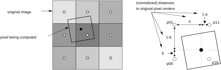
The influence of a neighboring pixel depends on the distance between its center and the center of the resulting pixel. Therefore, first the horizontal and vertical distances of the transformed coordinates to the adjacent pixel centers are determined.
The resulting gray value is computed as follows:
With \(h_{\rm res}\) denoting the gray value of the resulting pixel and \(h_{\rm ij}\) denoting the gray values of the neighboring pixels.
In this case, the resulting gray value is influenced by the gray values of all four neighboring pixels, bilinear interpolation produces smoother images than nearest neighbor interpolation but it also requires longer computation times.
Bilinear interpolation with integrated smoothing🔗
If the image transformation includes a downscaling of the image, so-called aliasing effects can appear. These effects result from a loss of information and may produce undesired artifacts in the downscaled image. To reduce the effects of aliasing, the image must be smoothed before it is scaled down.
Equally weighted bilinear interpolation (‘constant’)🔗
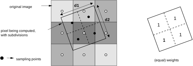
If ‘constant’ is selected, the gray values are determined using equally weighted bilinear interpolation.
Here the resulting pixel is subsampled, meaning, it is divided into multiple parts.
In the example below, the back-transformed resulting pixel has the size [1:5; 1:5] with respect to the pixels in the
input image.
It is sampled twice in each direction.
The gray value at each sample point is determined by bilinear interpolation in the input image. Finally, the
gray value of the resulting pixel is computed by calculating the mean of the gray values of all sample points.
Gaussian-weighted bilinear interpolation (‘weighted’)🔗
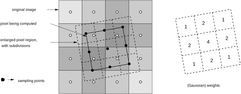
If ‘weighted’ is selected, the gray values are determined using Gaussian-weighted bilinear interpolation. Here the gray value interpolation is executed in three steps:
- subsampling
- determination of the gray values of the sample points
- calculation of the resulting gray value from the gray values of all sample points
The interpolation method ‘weighted’ roughly corresponds to smoothing the image with a Gaussian filter before
subsampling.
Compared to equally weighted bilinear interpolation, this interpolation method produces output
images with a smoother appearance but the runtime increases significantly for downscaled images.\
The main difference is that here an area larger than the pixel is divided into more subpixels.
The determination of the gray value of each sample point is carried out in the same way as for the method ‘constant’ by bilinear interpolation.
However, in contrast to equal weights used for the method ‘constant’, now a Gaussian smoothing is applied.
The example shows the weighting for the case that the resulting pixel is sampled at 3x3 positions.
Bicubic interpolation (‘bicubic’ and ‘bicubic_clipped’)🔗
If ‘bicubic’ is selected, the gray values are determined using bicubic interpolation.
It considers a weighted average of 16 pixels surrounding the closest corresponding pixel in the
image.
Based on the gray values of these 16 pixels a bicubic polynomial surface is constructed. This surface is
then used to determine the gray value at the requested (sub-)pixel position.
This produces smoother interpolation results and leads to fewer interpolation artifacts compared to ‘bilinear’ or ‘nearest_neighbor’ interpolation.\
Bicubic interpolation may lead to unexpected results due to aliasing if the image is downscaled. To reduce these undesired effects, an interpolation method with integrated smoothing should be used if a high quality of downscaled images is required.
Note
The resulting gray values may lie outside of the gray value range of the given image. If the interpolation method ‘bicubic_clipped’ is selected, these gray values are clipped to the gray value range of the input image. This method is only available for the determination of gray values at specific positions.
Influence of the system parameter int_zooming🔗
Another way to influence quality and speed of gray value interpolation is given by the system parameter int_zooming.
This parameter determines if image transformations are performed with integer arithmetic or with
floating point arithmetic.
For int_zooming set to true, the transformation is carried out internally using fixed point arithmetic. This leads to much shorter execution times.
However, it slightly decreases the accuracy of the transformed gray values. Also, for some operators, pixels with undefined gray values can occur.
In some cases the domain region can slightly differ as well, depending on int_zooming.
If ‘int_zooming’ is set to false, the transformation is carried out with floating point arithmetic. This results in more accurate calculations.
For byte images, the differences between both calculations is typically less than two gray levels. Correspondingly, for int2
and uint2 images, the gray value differences can be as large as 512 gray levels if the entire dynamic range of 16 bit
is used.
The value of int_zooming is set to true by default. To change this value, the operator set_system can be used.
The system parameter int_zooming affects the following operators regarding geometric transformations of
images:
projective_trans_imageprojective_trans_image_sizeaffine_trans_imageaffine_trans_image_sizepolar_trans_image_extpolar_trans_image_invrotate_imagescale_imagezoom_image_factorzoom_image_size
Runtime comparison🔗
Important
The runtime factors may vary depending on the downscaling factor and your hardware.
Runtime comparison for image transformation methods🔗
| Interpolation method | Quality | Runtime | Recommended usage |
|---|---|---|---|
| ‘nearest_neighbor’ | low | 1 | Only for time critical applications |
| ‘bilinear’ | high for upscaling | 3 | If downscaling doesn’t have to be slower than upscaling |
| ‘constant’ | enhanced for downscaling | 3 (upscaling) and 10 (downscaling) | If the image quality should be consistent for down- and upscaled images |
| ‘weighted’ | best for downscaling | 3 (upscaling) and 20 (downscaling) | If the image quality of downscaled images is critical for the application |
| ‘bicubic’ | very high for upscaling | 6 | If the image quality of upscaled imaes is critical for the application |
Runtime comparison for measure objects transformations and the determination of gray values at specific positions🔗
| Interpolation method | Quality | Runtime measure (relative to nearest_neighbor) | Runtime det. grey values (relative to nearest_neighbor) | Recommended usage |
|---|---|---|---|---|
| ‘nearest_neighbor’ | low | 1 | 1 | For time critical applications |
| ‘bilinear’ | low | 1.3 | 3 | Standard case |
| ‘bicubic’ | very high | 1.8 | 6 | For highest accuracy |
| ‘bicubic_clipped’ | very high | 1.8 | 6 | For highest accuracy |
Examples🔗
Rotation🔗
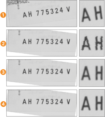
Here you see the results for ‘nearest_neighbor’, ‘bilinear’, and ‘bicubic’ interpolation, compared for a pure rotation without scaling of the image.
-
Displays the original image containing a serial number of a bank note, where the characters are not horizontal. The image is rotated so that the serial number is horizontal using the interpolation methods ‘nearest_ neighbor’, ‘bilinear’, and ‘bicubic’.
-
Displays the result of the rotation using ‘nearest_neighbor’ interpolation. In the detailed view, the typically undesired jagged appearance at the edges of the characters is clearly visible.
-
Displays the result of the rotation using ‘bilinear’ interpolation. The edges of the characters now have a very smooth appearance. This is due to the fact, that bilinear interpolation considers four neighboring pixels instead of only one for the determination of the resulting gray value. Note that the results of the interpolation methods ‘bilinear’, ‘constant’, and ‘weighted’ are the same for pure image rotations.
-
Displays the result of the rotation using ‘bicubic’ interpolation. For pure rotations without upscaling, the result is very similar to that of bilinear interpolation.
Upscaling🔗
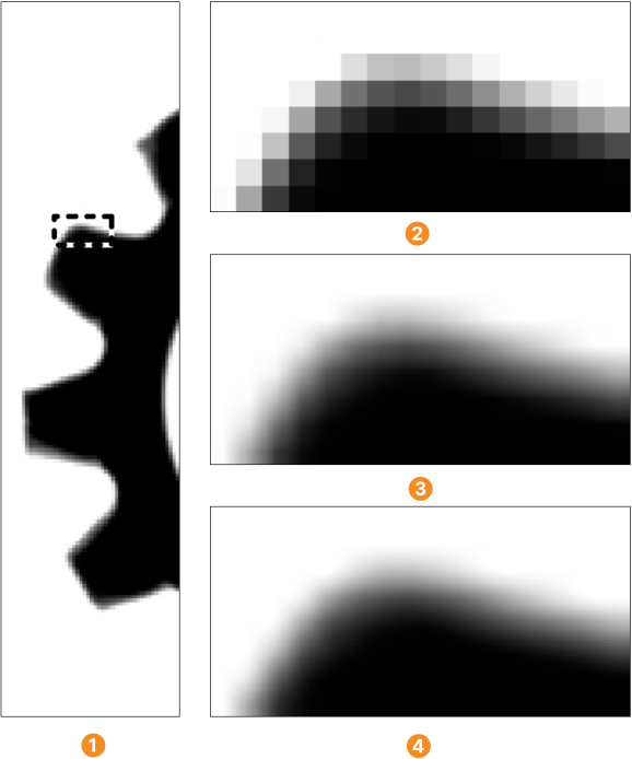
Here you see the effect of an image transformation that includes upscaling with a scaling factor of 10, comparing results for the interpolation methods ‘nearest_neighbor’, ‘bilinear’, and ‘bicubic’.
-
Displays the image to be transformed. It shows a part of a retainer.
-
Displays the result when using nearest_neighbor interpolation. The pixel structure of the original image is clearly visible. For a better presentation of the results, only enlarged views of the detail are shown.
-
Displays the result when using ‘bilinear’ interpolation. Although the edge appears much smoother, you can still perceive the pixel structure of the original image. The results of the interpolation methods ‘bilinear’, ‘constant’, and ‘weighted’ are the same for upscaling.
-
Displays the result when using ‘bicubic’ interpolation. The edge appears nearly perfectly smooth. The pixel structure of the original image is no longer visible.
Downscaling🔗
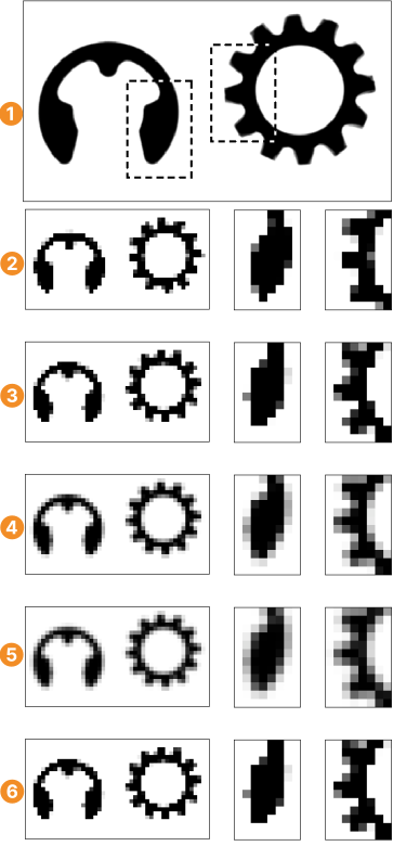
Here you see the effect of an image transformation that includes downscaling with a scaling factor of 0.1. With the compared results for the interpolation methods ‘nearest_neighbor’, ‘bilinear’, ‘constant’, ‘weighted’, and ‘bicubic’.
-
Displays two objects, a security ring on the left side and a retainer on the right side. For a better presentation of the results, a detailed view of each object is given for every interpolation method.
-
Displays the result of downscaling the image using ‘nearest_neighbor’ interpolation. The result of this massive downscaling is of poor quality. Especially in both detailed views, the shapes are often nearly straight whereas the shapes at the same part in the original image are completely different and with roundings.
-
Displays the result of downscaling the image using ‘bilinear’ interpolation. The quality is slightly improved compared to nearest_neighbor interpolation, but there are still heavy distortions in the shapes of the objects.
-
Displays the result of downscaling the image using ‘constant’ interpolation. The downscaled image has a much smoother appearance and the shapes of the objects are similar to the ones in the original image. The quality of the downscaled image is significantly better compared to ‘bilinear’ interpolation.
-
Displays the result of downscaling the image using ‘weighted’ interpolation with an integrated Gaussian filter. The image is still smoother compared to ‘constant’ interpolation and the shapes are nearly true to original. In the detailed view you can see, that the gradation of the edges is also finer. Thus, the result of ‘weighted’ interpolation provides the best quality for image transformations that include downscaling.
-
Displays the result of downscaling the image using ‘bicubic’ interpolation. For downscaling, the result is very similar to that of ‘bilinear’ interpolation.