Optimization for compute devices🔗
Tips and tricks for optimizing the usage of compute devices🔗
Speedup🔗
Since many aspects influence whether using compute devices can improve speed, the only way to know for certain which is faster, processing on CPU or on CPU and compute device, is to compare the execution times. However, there are quite a few aspects that may help to improve the speedup or influence the decision whether or not an application benefits from the use of compute devices. These aspects will be presented in the following sections as well as an example of how execution times can be compared quickly.
Requirements for improving speed with compute devices🔗
The highest speedup can be achieved by
- using a high-end graphics card,
- using hardware with high memory bandwidth, and
- creating a well structured program (group compute device operations to minimize transfer between CPU and compute device).
Memory transfer can be measured with the hbench option (-memory).
Note that HALCON’s operators are automatically parallelized. This means that the available CPU cores are recognized and the threads are then automatically divided without the need for the programmer to interfere. This way, the speed increases proportionally to the number of processors since operators with AOP are significantly faster. Therefore it is very important to compare CPU and compute device performance on the same hardware that will be used in the subsequent application.
Aspects to be considered🔗
Note that the transfer of data between CPU and compute device is a bottleneck. Using compute devices may only be an efficient solution if the whole application is faster, i.e., execution time plus transfer time.
Note also that the energy consumption of a graphics card is very high. Graphics cards may also not be designed for use in an industrial environment. Therefore problems concerning the graphics cards may be:
- They might not be robust against heat or vibrations.
- They may not correct memory errors (ECC).
- They may only perform single-precision floating point operations.
Other aspects that should be considered concerning the transfer are:
- Transfer rate is usually larger for large block sizes.
- Transfer is usually faster when using page locked (pinned) memory (i.e. memory with a fixed address that can be set via
set_compute_device_param).
Using compute devices does not always improve speed🔗
It is unlikely that transferring calculations to the compute device will improve speed if
- the CPU is already very fast,
- fast operators are used,
- the transfer times are slow because of
- memory bandwidth or
- large images.
The influence of image size on speed🔗
Improving the speed of calculations works most efficiently for large images. Benchmarks have shown that images with a width that can be divided by four can be calculated faster. Therefore, the performance can be optimized if an image is either cropped or enlarged such that the width is a multiple of 4 byte, or even better 16 byte, before it is processed on the compute device.
Note, however, that for some operators performing geometric transformations, the image will be calculated on the CPU instead of being transferred to the compute device if it is too large.
The operator get_compute_device_info can be used to query image width and height that is supported by the compute device.
Operators🔗
Operators that return sub-pixel precise XLD contours perform in two steps, filtering and extracting the XLD contours.
If calculations are executed on the compute device, the filtering is performed directly on the compute device. The filtered images are transferred back to the CPU for XLD extraction.
This transfer back to the CPU is relevant for the total execution time. For this reason, it is important to have a PC with high transfer rate between CPU- and compute device memory.
Allocating cache for maximum performance🔗
Two kinds of caches are used on the compute device, buffer (for filters like mean_image or sobel_amp) and images (for geometric transformations).
For maximum performance, we recommend to allocate those two kinds of cache before executing an operator.
Otherwise, the runtime will be higher since memory is allocated dynamically.
The default of those caches is one third of the available memory each (to change the maximum size of the compute device image cache, use set_compute_device_param (DeviceHandle, 'buffer_cache_capacity')).
Measuring execution times🔗
When using compute devices, processes on the compute device and on the CPU are performed asynchronously by default. A visualization of asynchronous processing can be found in Figure 1.
Asynchronous processing has many advantages:
- Operators that are processed on the CPU do not have to wait for the compute device operators.
- CPU and compute device process in parallel.
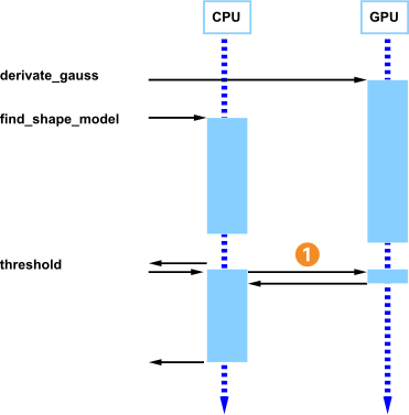
Start transfer
However, due to the asynchronous processing even though the general execution time may decrease, the execution time of single operator may not be measured correctly because an operator might for another one. Therefore, to get the exact execution times, asynchronous processing has to be turned off.
Using synchronous processing for test purposes🔗
If synchronous processing is required, e.g., if execution time of a single operator should be measured with set_compute_device_param, the generic parameter DeviceHandle 'asynchronous_execution' should be set to 'false'.
Note however that for measuring the execution time of an application, the default setting 'true' should be used to achieve the best performance.
The example compute_devices.hdev shows how to perform a benchmark and how to make sure that the image is really transferred to the compute device and therefore if the transfer time is included in the time measurements.
Exchanging or simulating operators that do not support compute devices🔗
Some operators that do not support compute devices can be simulated by other operators.
Use the operator convol_image to replace linear filters like
laplace,bandpass_image,- or any other arbitrary filter mask.
Processing domains and regions🔗
All compute devices that are addressed via OpenCL are optimized for the processing of images not regions. Therefore the domain cannot be used to reduce the area to which the operator is applied. The main reason for this is that the whole image needs to be transferred to the compute device.
These operators are
binomial_filterconvol_imagederivate_gaussmedian_imagesobel_ampsobel_dirlines_gaussedges_imageedges_sub_pix
To reduce transfer and execution times of images with reduced domains as far as possible, crop the image,
e.g., with the operator crop_domain
before they are transferred to the compute device.
Note that, depending on the filter size of the operator to be executed, the domain of the image should be suitably enlarged before the call of crop_domain.
Simulating region processing🔗
In this paragraph, the simulation of region processing is shown for the example of color segmentation.
Color segmentation can be sped up by using compute devices instead of just the CPU.
In order to calculate the complete color segmentation on a compute device and therefore reduce transfer time, region processing has to be simulated.
This is done by creating binary images, i.e., images with exactly two gray values.
In the following example, these gray values are 0 and 255.
Pixels with a gray value of 0 are defined as outside of the region whereas pixels with a value of 255 are recognized as within the region.
Therefore regular morphology operators (like, e.g., dilation_rectangle1) can be replaced by gray-value morphology operators (like, e.g., gray_dilation_rect).
In the example below, the blue plastic part of a fuse should be detected. This example first shows which operator calls solve this problem on the CPU and then which operators are used for the same solution on a compute device. reffig{gpu.simulate.threshold} shows the results of each step of the region processing on the CPU compared to the results of simulated region processing on a compute device.
| Step | CPU | Compute device |
|---|---|---|
| 0 |  |
|
| 1 |  |
 |
| 2 |  |
 |
| 3 |  |
 |
| 4 |  |
 |
read_image (ColorFuses00, 'color/color_fuses_00.png')
decompose3 (ColorFuses00, Image1, Image2, Image3)
First, an image is read. For further processing, the three-channel image is converted into three images.
The image is subsequently transformed into the color space 'hsv' with the operator trans_from_rgb.
Then the region is processed on the CPU.
For this purpose, regions with a certain hue and saturation are selected (see Table 1, steps 1 and 2).
trans_from_rgb (Image1, Image2, Image3, Hue, Saturation, ImageResult3, 'hsv')
threshold (Hue, Region, 125, 145)
threshold (Saturation, Region1, 100, 255)
Now to combine the two regions, the intersection of the two resulting regions of the thresholds is calculated (see Table 1, step 3).
To reduce this region to the blue plastic part of the fuse, the morphology operators dilation_rectangle1 and erosion_rectangle1 are used (see Table 1, step 4).
Now the upper part of the blue fuse can be determined.
intersection (Region, Region1, RegionIntersection)
dilation_rectangle1 (RegionIntersection, RegionDilation, 11, 11)
erosion_rectangle1 (RegionDilation, RegionErosion, 91, 31)
dilation_rectangle1 (RegionErosion, RegionDilation1, 81, 21)
The same process can be simulated on a compute device.
A fast solution to start processing color images on a compute device is to transfer the Bayer image to the compute devices where the operator cfa_to_rgb can be executed to transform it into a color image.
Only a subset of the color space transformations can be processed on the compute device with trans_from_rgb (as shown in this example) and trans_to_rgb.
trans_from_rgb (Image1, Image2, Image3, Hue, Saturation, ImageResult3, 'hsv')All other color space transformations can be simulated with linear_trans_color.
If the color in an image changes, this effect can be corrected by modifying TransMat as explained in the reference documentation of linear_trans_color.
Instead of using a threshold like on the CPU, the image is scaled such that all pixels belonging to the object are mapped to the gray value 255 and all that are outside of the object are mapped to 0. To speed up this mapping, a LUT transformation is applied. Two look-up tables are used for further processing.
The first LUT maps three gray-value ranges. The values
- 0 to 124 are mapped to 0,
- 125 to 145 are mapped to 255, and
- 146 to 255 are mapped to 0.
LUT_125_145 := [gen_tuple_const(125,0),gen_tuple_const(21,255), gen_tuple_const(110,0)]The second LUT maps two gray-value ranges. The values
- 0 to 99 are mapped to 0 and
- 100 to 255 are mapped to 255.
LUT_100_255 := [gen_tuple_const(100,0),gen_tuple_const(156,255)]The result of using the defined LUTs with the operators lut_trans for hue and saturation are two byte images with only two different gray values: 0 and 255 (see Table 1, steps 1 and 2).
lut_trans (Hue, HueThresh, LUT_125_145)
lut_trans (Saturation, SaturationThresh, LUT_100_255)
By calculating the minimum of both images and using the two gray-value morphology operators gray_dilation_rect and gray_erosion_rect, the blue plastic part of the fuse can be determined (see Table 1, steps 3 to 4).
min_image (HueThresh, SaturationThresh, ImageIntersection)
gray_dilation_rect (ImageIntersection, ImageMax, 11, 11)
gray_erosion_rect (ImageMax, ImageMin, 31, 91)
gray_dilation_rect (ImageMin, ImageMax1, 21, 81)
Note that it must be considered that the runtime of gray-value morphology operators increases with the size of the filter masks whereas operators like opening_rectangle1 that perform region morphology have a constant runtime that is independent from the size of the structuring element.
Operators using regions like union2, intersection, and difference are simulated on the compute device with the operators max_image, min_image, and sub_image if the regions are represented as binary images.
Limitations of compute devices🔗
For other operators, only certain parameters may be supported for being processed on a compute device. A few examples are listed here:
median_image can only be used with filter mask sizes 3x3 and 5x5
derivate_gauss can only be used with a limited number of filters and maximum smoothing with sigma 20.7 (depending on the filter this value can even be lower),
trans_from_rgb can only be used for color spaces ‘cielab’, ‘hsv’ and ‘hsi’.
These are just some examples for limitations.
Note
Remember to always check which parameter settings are available for an operator that is processed on a compute device.
If only a certain subset of values is available for a parameter, this information is listed just beneath the regular values under List of values (for compute devices).
For more information on limitations, please refer to this page.
Using one compute device🔗
Limitations of compute devices🔗
For other operators, only certain parameters may be supported for being processed on a compute device. A few examples are listed here:
median_imagecan only be used with filter mask sizes 3x3 and 5x5derivate_gausscan only be used with a limited number of filters and maximum smoothing with sigma 20.7 (depending on the filter this value can even be lower),trans_from_rgbcan only be used for color spaces'cielab','hsv'and'hsi'.
These are just some examples for limitations.
hAttention{Remember to always check which parameter settings are available for an operator that is processed on a compute device.}
If only a certain subset of values is available for a parameter, this information is listed just beneath the regular values under List of values (for compute devices):.
For more information on limitations, please refer to the refManual{keyHInstallGuide}[ (in refsec{developinglimitationsgeneral})].
Multithreading🔗
Using one compute device🔗
To use one compute device in different threads, the compute device needs to be opened in each thread separately. Thus, one compute device is represented by different compute device handles. Note that each compute device handle is treated as a separate device and cannot access data stored on the other ‘devices’ without copying to the CPU first.
We do not advice to use one compute device in multiple threads, because you need a lot of synchronization logic to make sure that the compute device is not used simultaneously by another thread, and that the results are shared correctly between threads. Thus, you may end up with a complicated code.
If you look at the operator reference of, for example, activate_compute_device under the heading “Execution Information”, you will see that the multithreading scope is local.
This means that compute device operators must only be called from the thread that created the compute device handle, and compute device handles must not be shared across threads.
Note, however, if you try to access the same image object from different threads using the same compute device, an error will be raised.
Using more than one compute device🔗
Note
If planning to use more than one compute device, it should be checked whether the PC hardware is able to handle this. It is important to always install the latest graphics driver. If the compute device is accessed via a Linux system, the user must be member of the ‘video’ group.
By default only one compute device is used if the compute device is activated with activate_compute_device.
If another compute device has been activated previously, this compute device is automatically deactivated for the current thread.
It is, however, possible to use more than one compute device. Then, one thread per device must be used. Each thread connects to its compute device and starts processing. Since this does not cost much execution time, all threads can run on the same CPU.
Technical details🔗
Please refer to the websites of NVIDIA, ATI/AMD and Intel for a list of compatible cards.
To check the performance of a card, it is useful to measure the runtimes and transfer times which can be done via hbench - compute_device [-ref] or like shown in this programming example.
The following technical characteristics should be taken into account when considering to use compute devices:
-
Power/Performance Ratio In some applications the power consumption and/or the emitted heat is of importance. It can therefore be useful to compare different cards with respect to their performance and consumed power.
-
Robustness It is useful to check whether a compute device was designed for industrial use.