Advanced topics for texture analysis🔗
Fast Fourier transform (FFT)🔗
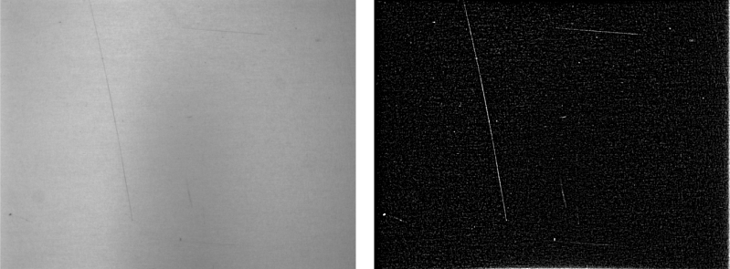
Fast Fourier transform, short FFT, is another option for texture analysis. This method makes use of the different frequencies in textures. HALCON’s FFT exactly determines the amount of each frequency in the image. It enables the construction of any type of linear filters which means that application-oriented filter designs are possible. There is also a huge set of predefined filters as well as advanced Gabor texture filters. With HALCON’s FFT it is possible, e.g., to emphasize any structure of a special texture (see Figure 1). A convolution can be performed by transforming the image and the filter into the frequency domain, multiplying the two results, and transforming the result back into the spatial domain. Therefore the two reasons for using FFT are:
- For bigger filter sizes it is more efficient to apply the filters in Fourier domain as FFT always takes the same time for any mask size, unlike normal filters.
- It is a great advantage that filters can be customized to remove or emphasize specific frequencies from the image.
Standard operators for FFT are:
fft_generic: a generic version of the complex Fourier transform,rft_generic: real-valued Fourier transform,fft_image, a shortcut for the forward transformation withfft_generic- and
fft_image_inv, a shortcut to the backward transformation withfft_generic.
About texture features🔗
Entropy and anisotropy🔗
Entropy and anisotropy describe the gray value distribution of an image independent of the position of the pixels.
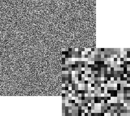
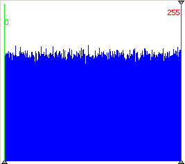
The entropy for white noise, as shown in Table 1 (left), is high as white noise comprises of an equal number for all gray values.
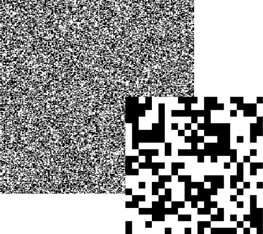
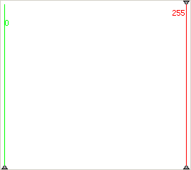
Even though binary noise Table 1 (center) looks similar to white noise at first sight, it is in fact quite different because it only consists of two gray values: black and white. Therefore, the entropy is very low.
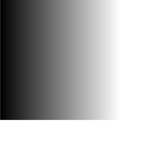
Image Table 1 (right) shows a gray ramp which has the same value for entropy than the white noise image even though they look very different. Both images include, however, the same frequency for each gray value. This shows that the position of pixels within an image has no influence on the image’s entropy.
| White noise | Binary noise | Gray value ramp |
|---|---|---|
 |
 |
 |
 |
 |
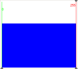 |
| entropy = 8 | entropy = 1 | entropy = 8 |
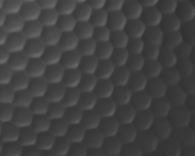
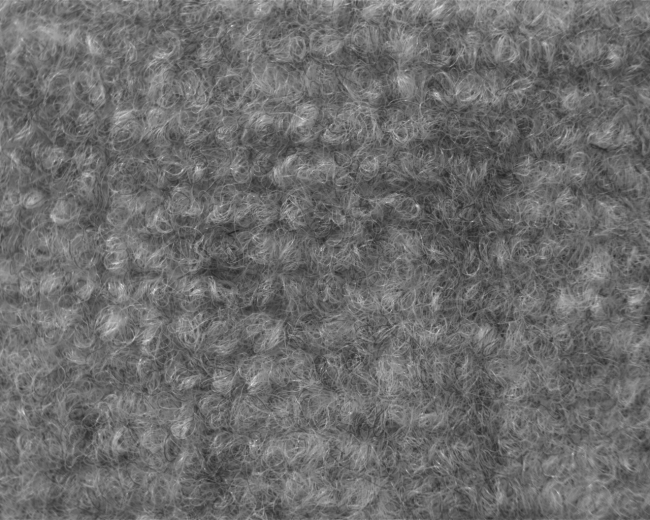
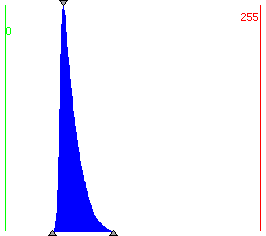
Even though real images do not usually show such extreme values, the examples in Table 2 still highlight the connection between gray value distribution (as is presented in the histogram) and the entropy value.
Example images for entropy values
| Honeycomb structure | Dust filter |
|---|---|
 |
 |
 |
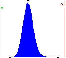 |
| entropy = 5.12 | entropy = 6.40 |
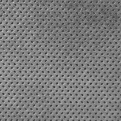
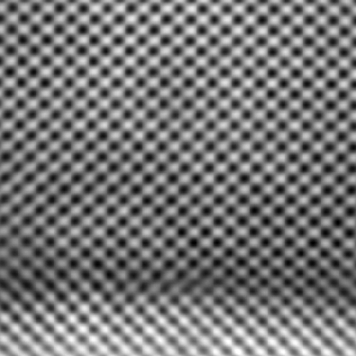
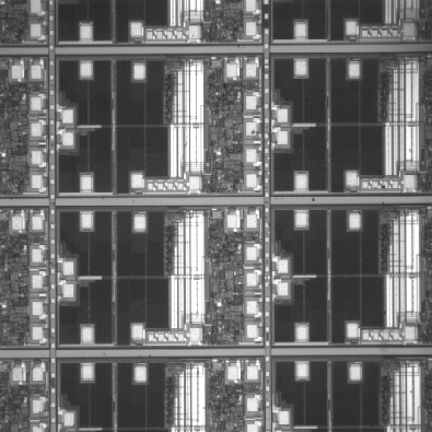
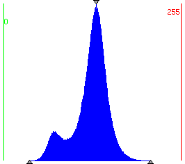
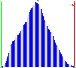
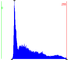
Anisotropy determines the symmetry of the gray value distribution. A value of -0,5 means that the histogram curve is symmetric. The value is higher if the image has more bright parts and lower if it has more dark parts as becomes clear from Table 3.
Example images for anisotropy values
 |
 |
 |
|---|---|---|
 |
 |
 |
| anisotropy = -0.55 | anisotropy = -0.50 | anisotropy = -0.40 |
Cooccurrence matrix🔗
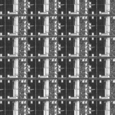
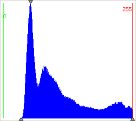
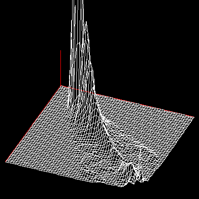
The cooccurrence matrix describes the relationship between the gray value of a pixel and the gray values of its neighbors. The matrix elements contain the probability that two gray values appear next to each other. Slow gray value changes are indicated by high values along the diagonal of the principal axis. Strong contrasts lead to entries far away from the diagonal of the principal axis. The connection between gray values in the image, in the histogram, and finally in the cooccurrence matrix is shown in Table 4. Computing the cooccurrence matrix, you can select which neighbors are evaluated. Based on the cooccurrence matrix, four features can be computed:
- Energy
- Correlation
- Homogeneity
- Contrast
 |
 |
 |
|---|---|---|
| Original image | Gray value histogram | Cooccurrence matrix |
Features of the cooccurrence matrix🔗
Energy
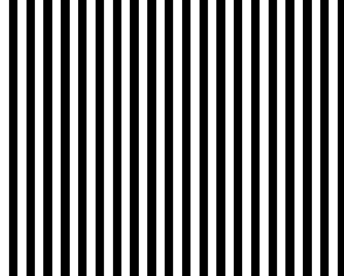
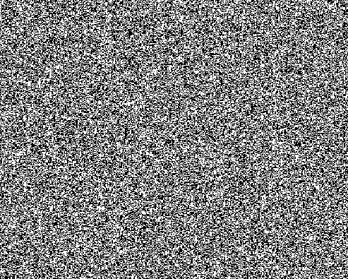
Energy is actually the short form for uniformity of energy and indicates if all kinds of gray value combinations are present or if certain gray value combinations are dominant. An image with a constant gray value has the highest energy.
 |
 |
| energy = 0.45 | energy = 0.0002 |
has a high energy because there are only few gray value combinations, which change always according to the same scheme. has little energy because the changes between pixels differ, i.e., there is no uniformity.
 |
 |
| energy = 0.088 | energy = 0.005 |
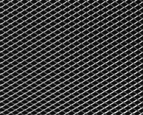
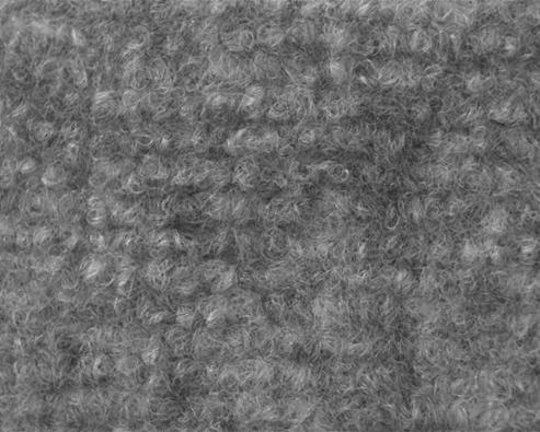
The textures in Table 6 show how parts that contain pixels of the same gray value contribute to the higher energy of , whereas gray values in are almost constantly changing and therefore lead to a low energy.
Correlation
Correlation defines the measure of dependency between neighboring values. If the matrix shows a thin line from top left to right bottom, this means that the image is blurry, which is why the values are so close together. A wide, roundish progress indicates a focused image. Contrasts and little or no correlation are indicated by pixels far away from the main diagonal. The question of correlation between pixels can however sometimes depend on the image’s orientation as is depicted in Table 7.
|
 |
 |
| original image | correlation 0° = -1.0 | correlation 90° = 1.0 |
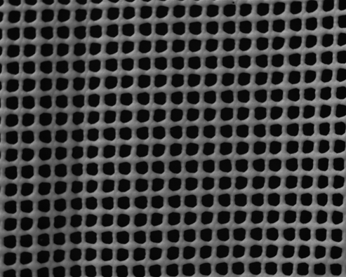
The two correlation values of the same image are very different depending on the rotation of the image. 0° causes a low correlation whereas 90° has a high one. In Table 8 the correlation values show that with extreme gray value changes has a lower value than with a texture that consists of gray values which are quite similar to each other.
 |
|
| energy = 0.0959 | energy = 0.795 |
Homogeneity
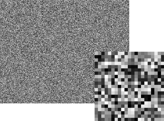
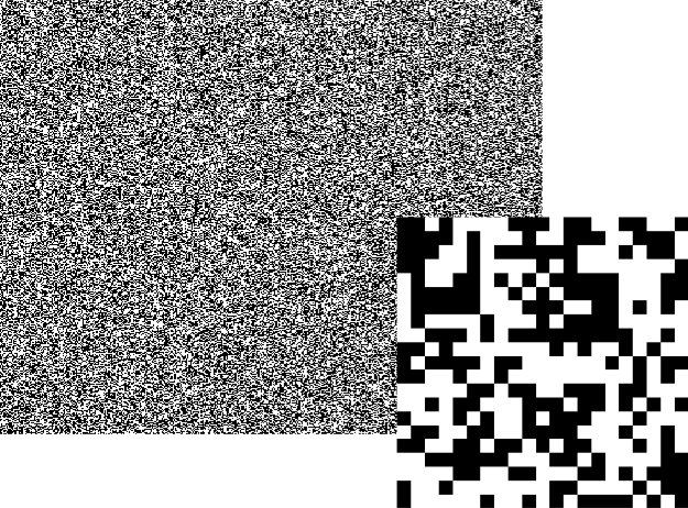
Homogeneity is high if large areas in an image have the same gray values.
 |
 |
| homogeneity = 0.47 | homogeneity = 0.5 |
does not include any groups of pixels with the same gray values which makes it very inhomogeneous. with white noise includes areas, a feature which makes it more homogeneous. A unicolored image has the highest homogeneity value.
|
 |
| homogeneity = 0.65 | homogeneity = 0.66 |
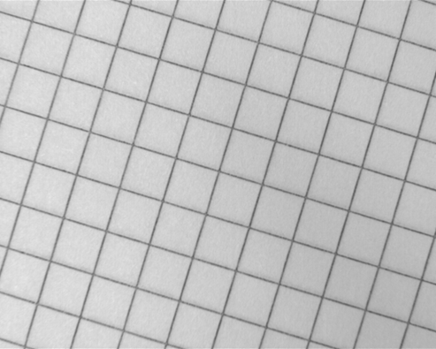
Realistic images, as shown in Table 10, clarify these homogeneity rules. Even though both images look partially homogeneous (they both contain bright and dark parts of a certain size but also include some changes from dark to bright) there are little differences. The mesh image is less homogeneous because the structure is three dimensional and therefore little deviations in brightness can cause slightly different gray values on the white mesh. , however, contains bigger parts with a same gray value (the white background) and is also only two dimensional.
Contrast
The contrast value between two pixels is multiplied and squared. High differences lead to steep edges and a high value.
|
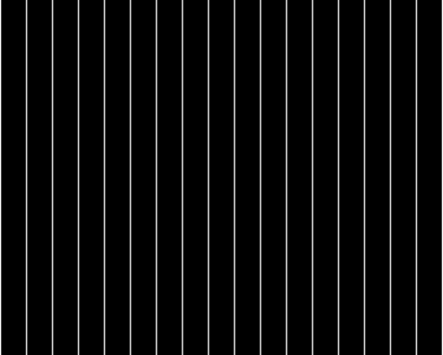 |
| contrast = 3969 | contrast = 203.9 |
The example images in Table 11 depict lines that run in different distances from each other. The image with the denser lines also has a higher contrast. This shows that the contrast value includes the frequency as well as the intensity.
|
|
| energy = 0.088 | energy = 0.005 |
In Table 12, the grid structure in has a higher contrast than the dust filter in because the gray value changes in are more extreme than the gray value changes in .
About texture filters🔗
About the laws filter🔗
By applying a Laws filter, you can enhance or suppress textural structures in an image based on their spatial frequency, i.e., the size of the texels.
The operator texture_laws applies texture transformations according to K. I. Laws) to an image.
This is done by convolving the input image with a special filter mask of either 3x3, 5x5, or 7x7 pixels.
For most of the filters the resulting gray values must be modified by a shift.
This makes the different textures in the output image more comparable to each other, provided suitable filters are used.
The name of the filter is composed of the letters of the two vectors used, where the first letter specifies a convolution in the column direction, while the second letter specifies a convolution in the row direction. The letters themselves specify the convolution. You can select “l”, “e”, “s”, “r”, “w”, “o” with “l” emphasizing low and “o” emphasizing high frequencies.
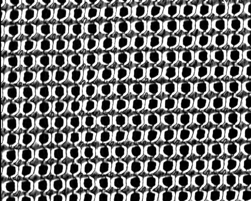
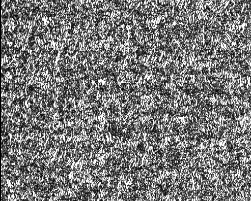
Therefore, the second letters detecting low frequencies to high frequencies are “l”, “e”, “s”, “r”, “w” and “o”. The example figures Table 13 and Table 14 show how the two common texture filters “le” and “ls” work on two different textures.
|
 |
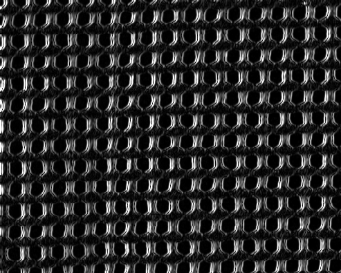 |
The Laws filter “le” looks for low frequencies in the image. As can be seen in Table 13, there are a few low frequencies in the image. The Laws filter “ls”, however, looks for high frequencies, which occur very rarely in the image in places where gray values change from black to white and vice versa. As a result, the filtered image looks quite dark.
|
 |
 |
The filtered images in Table 14 show that the original image contains low frequencies as well as high frequencies as it responds to both the “le” and “ls” filter. The Laws filter is therefore useful to distinguish textures which differ in their frequencies in a certain direction.