Gray value morphology🔗
Gray value morphology provides a set of operators that allow the
Unlike the binary operations described in Region morphology, morphological gray value operators deal with input images that contain pixels with a range of more than one bit. Therefore, gray value morphology can be seen as a generalization of region morphology.
Dilating or eroding a grayscale image🔗
To perform a dilation or erosion, each pixel of the image is assigned a gray value depending on its neighborhood.
Area and shape of the neighborhood affecting each pixel are defined by the chosen
Implementing a dilation, every pixel of the input image is assigned the maximum gray value of its neighborhood.
Consequently, for an erosion, the minimum gray value is assigned.
Accordingly, bright areas of the input image are enlarged by gray value dilation, whereas gray value erosion emphasizes dark areas.
 |
 |
 |
 |
Figure 1.
Original gray value image
Structuring element with reference point in the origin
Result of eroding the input image
Result of dilating the input image
Table 1 shows the operators that can be used to dilate or erode an image.
| Morphological operator | Structuring element | |
|---|---|---|
gray_dilation |
gray_erosion |
arbitrary |
gray_dilation_rect |
gray_erosion_rect |
rectangular |
gray_dilation_shape |
gray_erosion_shape |
rhombus, rectangle, octagon |
Morphological grayscale operations are often part of the preprocessing of images before information can be extracted properly. The following example displays a case where a gray value erosion is necessary to read data code symbols.
Example
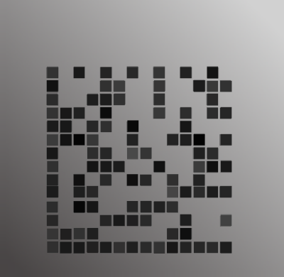
To fit a data model used for decoding, the gaps between the code elements in the image need to be reduced by enlarging local minima in a square shape.
Hence, a gray value erosion is performed, using an adequately sized rectangle as the structuring element.
The rectangle size depends on the data model created with create_data_code_2d_model, where the acceptable module gap size is determined.
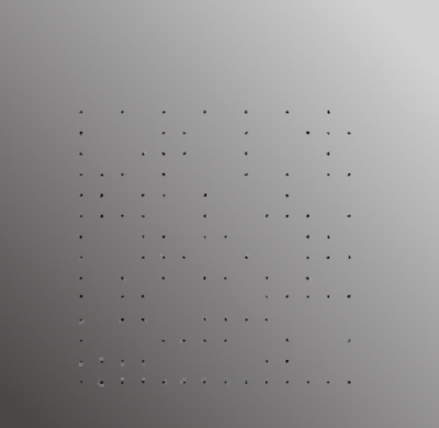 |
 |
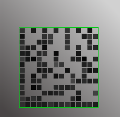 |
Figure 2.
Image of coded object
Erosion with square structuring element
Applying data model for decoding
(images from the example program 2d_data_codes_minimize_module_gaps.hdev)
Opening or closing a grayscale image🔗
Gray value opening and gray value closing operators each are a combination of the operators explained above.
Closing is a dilation followed by an erosion, while opening is an erosion followed by a dilation operation.
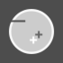
As shown in the example images blow, gray_closing reduces or even removes parts of the image that are darker than their neighborhood, whereas gray_opening reduces lighter areas.
Furthermore, using a suited structuring element, you can preserve shapes while removing unwanted image artifacts.
 |
 |
 |
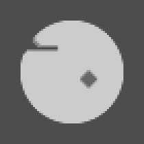 |
Figure 3.
Original gray value image
Structuring element with reference point in the origin
Result of closing the input image
Result of opening the input image
Further operators🔗
To take a closer look at areas that are affected by gray value opening or closing, you can perform a gray_tophat or gray_bothat transformation.
The resulting image displays the difference between the original image and the opening respectively closing of an image.
You can also use these operators to detect structures that match the shape of the structuring element.
The gray_range_rect operator gives you the opportunity to detect fine structures on homogeneous surfaces by visualizing the extent of local variations in pixel values.
 |
 |
 |
Figure 4.
Top hat
Bottom hat
G ray value range
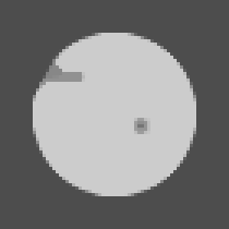
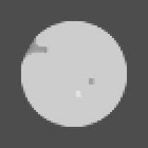
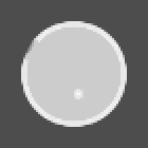
By applying the gray_range_rect operator, you can perform a mitigated form of a gray value opening or closing operation.
You can control the transformation by adjusting the parameter ModePercent.
 |
 |
 |
 |
 |
Figure 5. Dual rank operations:
ModePercent = 0 (equals opening)
ModePercent = 25
ModePercent = 50 (equals median)
ModePercent = 75
ModePercent = 100 (equals closing)