Workflow🔗
Shape-based 3D matching consists of the following basic steps:
-
the 3D object model is accessed from file,
-
the 3D shape model is created from it, and
-
the 3D shape model is used to search the object in search images.
An example for the shape-based 3D matching of tile spacers is the HDevelop example program %HALCONEXAMPLES%\hdevelop\3D-Matching\Shape-Based\create_shape_model_3d_lowest_model_level.hdev.
Step 1: Read the 3D object model
The 3D object model describing the search object is loaded in HALCON with the operator read_object_model_3d.
It must be available as a CAD model in one of the supported formats, for example, DXF, STL, or PLY.
The list of supported CAD formats and tips on how to obtain a suitable model, including the specification of the requirements the CAD models must fulfill, are provided with the description of the operator in the operator reference.
For additional tips on handling selected CAD formats, please contact your local sales partner.
read_object_model_3d ('tile_spacer.dxf', 0.0001, [], [], ObjectModel3DID, DXFStatus)Step 2: Create the 3D shape model
The 3D shape model is created with the operator create_shape_model_3d.
It needs the 3D object model and camera parameters as input.
Additionally, a set of parameters has to be adjusted.
The camera parameters can be obtained by a camera calibration.
In the example, the camera parameters are known and just assigned to the variable CamParam.
Before creating the 3D shape model, it is recommended to prepare the 3D object model for the shape-based 3D matching using prepare_object_model_3d.
Otherwise, the preparation is applied internally within create_shape_model_3d, which may slow down the application if the same 3D object model is used several times.
gen_cam_par_area_scan_division (0.0269462, -354.842, 1.27964e-005, 1.28e-005, 254.24, 201.977, 512, 384, CamParam)
prepare_object_model_3d (ObjectModel3DID, 'shape_based_matching_3d', 'true', [], [])
create_shape_model_3d (ObjectModel3DID, CamParam, 0, 0, 0, 'gba', -rad(60), rad(60), -rad(60), rad(60), 0, rad(360), 0.26, 0.27, 10, 'lowest_model_level', 3, ShapeModel3DID)
The 3D shape model is generated by computing different views of the 3D object model within a user-specified pose range. The views are obtained by placing virtual cameras around the object model and projecting the 3D object model into the image plane of each camera position. The resulting 2D shape representations of all views are stored in the 3D shape model.
An important task is to specify the pose range. To ease this task, imagine a sphere that surrounds the object. On the surface of the sphere, a camera is placed that looks at the object. Now, the pose range can be defined by restricting the position of the camera to a part of the sphere’s surface. Additionally, the minimum and maximum distance of the camera to the object, i.e., the radii of different spheres, must be specified.
In the following, the position of the sphere relative to the object and the definition of the surface part are described. The position of the sphere is defined by placing its center at the center of the object’s bounding box. The radius of the sphere corresponds to the distance of the camera to the center of the object. To define a specific part of the sphere’s surface, the geographical coordinates longitude (\(\lambda\)) and latitude (\(\varphi\)) are used (see ). For these, minimum and maximum values are specified so that a quadrilateral on the sphere is obtained (see ).
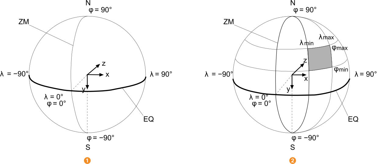
EQ: equator
ZM: zero meridian
To describe the orientation of the geographical coordinate system we introduce an object-centered coordinate system. This is obtained by moving the origin of the object coordinate system (CAD model) to the center of the sphere. The xz-plane of the object-centered coordinate system defines the equatorial plane of the geographical coordinate system. The north pole lies on the negative y-axis. The origin of the geographical coordinate system (\(\lambda\) = \(\varphi\) = 0°), i.e., the intersection of the equator with the zero meridian, lies in the negative z-axis.
To illustrate the above description, let us assume that we have the object model shown in . For illustrative purpose additionally the object coordinate system is visualized. In , the corresponding geographical coordinate system is shown together with a camera placed at its origin (\(\lambda\) = \(\varphi\) = 0°). Consequently, this camera view corresponds to a bottom view of the object.
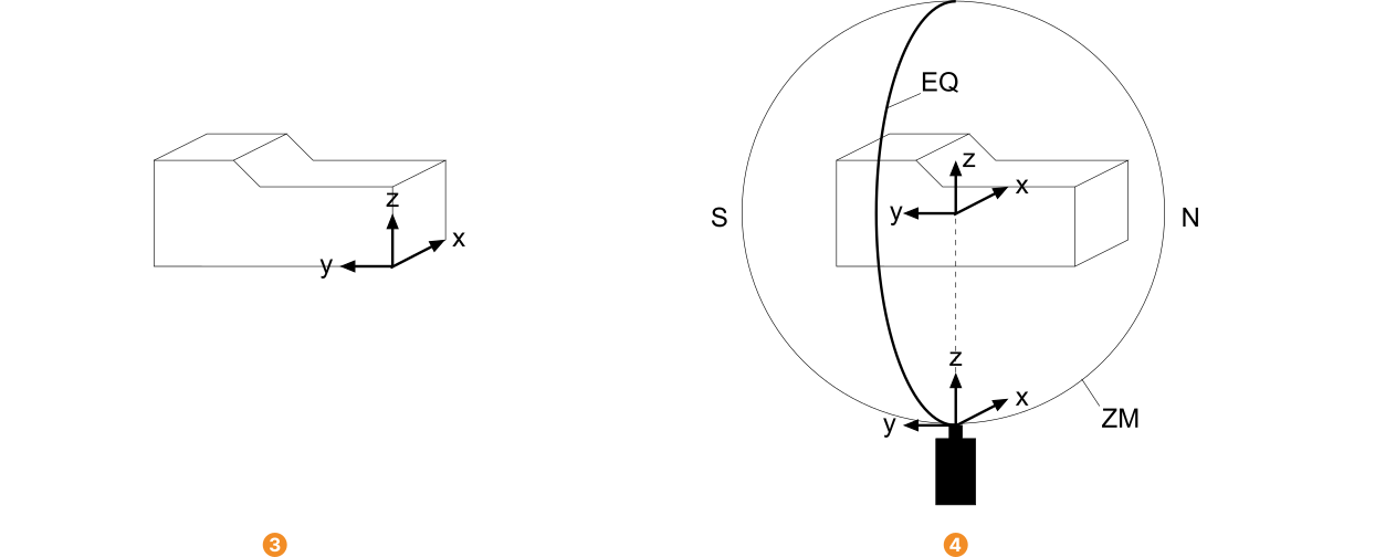
EQ: equator
ZM: zero meridian
Note that the coordinate system introduced here is only used to specify the pose range. The pose resulting from the shape-based 3D matching always refers to the original object coordinate system used in the CAD file and not to the center of the object’s bounding box.
In most cases, the specification of the pose range can be simplified by changing the origin of the geographical coordinate system (i.e., the orientation of the sphere) such that it coincides with a mean viewing direction of the real camera to the object.
This can be achieved by rotating the object-centered coordinate system, which defines the geographical coordinate system as described above.
The rotation can be specified by passing the rotation angles to the parameters RefRotX, RefRotY, and RefRotZ of the operator create_shape_model_3d.
That is, you can specify the pose range either by adjusting the longitude and latitude, leaving the origin of the sphere at its initial position, or by rotating the object-centered coordinate system to get a mean reference view and then specify the pose range in a more intuitive way (see Figure 3), which is recommended in most cases.
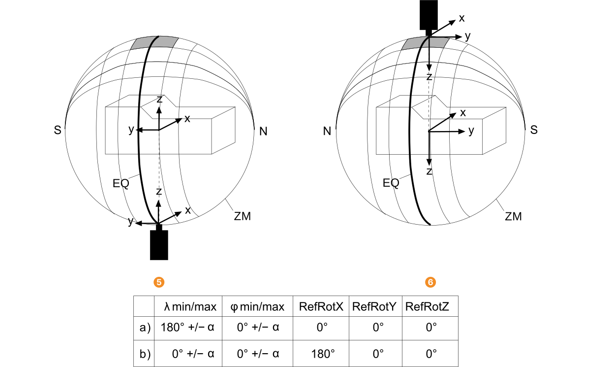
EQ: equator
ZM: zero meridian
Figure 4 shows a rotation-symmetric object, for which a reference view is specified. Rotation-symmetric objects have the specific advantage that they have the same appearance from all directions that are perpendicular to their rotation axis. Thus, if the mean reference view is selected such that the camera view is perpendicular to the rotation axis (and the rotation axis crosses the poles of the sphere), the longitude range can collapse to a single value so that the number of calculated 2D projections is significantly reduced. That is, less memory is needed and the matching becomes faster. Here, the initial z-axis of the object-centered coordinate system corresponds to the rotation axis of the object. To obtain the intended reference view, the orientation of the sphere is changed by rotating the object-centered coordinate system by -90° around its x-axis. Now, the pose range for \(\varphi\) is specified like described before and the pose range for \(\lambda\) is restricted to 0°.
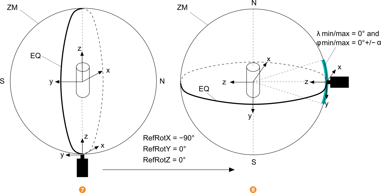
EQ: equator
ZM: zero meridian
Besides the definition of the pose range, also the camera roll angle, i.e., the allowed range for the rotation of the virtual camera around its z-axis, must be set.
In most cases, it is recommended to allow a full circle for the camera roll angle.
For details, we recommend to read the description of the operator create_shape_model_3d in the Reference Manual.
Step 3: Find the 3D shape model in search images
With the 3D shape model that was created by create_shape_model_3d or read from file by read_shape_model_3d, the object can be searched for in images.
For the search, the operator find_shape_model_3d is applied.
for I := 1 to NumImages by 1
    read_image (Image, 'tile_spacers/tile_spacers_color_' + I$'02')
    find_shape_model_3d (Image, ShapeModel3DID, 0.7, 0.85, 0, ['num_matches', 'max_overlap', 'border_model'], [3, 0.75, 'true'], Pose, CovPose, Score)
endfor
Several parameters can be set to control the search process. For detailed information, we recommend to read the description of the operator in the Reference Manual. The operator returns the pose of the matching model, the standard deviation of the pose, and the score of the found instances of the 3D shape model that describes how much of the model is visible in the image.