Using the matching results🔗
The main goal of matching is to locate objects in images, that is, above all get the position and in most cases also the orientation of a model instance in an image. Furthermore, many approaches return additional information like the scale of the object or a score that evaluates the quality of the returned object location.
About the results of the individual matching approaches🔗
To locate objects in images, information like the position and orientation of the searched objects must be returned by the matching.
This information is available in different representations, depending on the selected matching approach. For a strict 2D matching the position and orientation are returned separately, that is, the position consists of a row and a column value and the orientation consists of a single value describing the angle.
In contrast, the uncalibrated perspective approaches return the position and orientation together in a projective transformation matrix (2D homography) and the calibrated perspective approaches return them together in a 3D pose.
Besides the position and orientation, many approaches return further information like the scale of the found object or information about the quality of the match, which is called score.
Comparison of the matching approaches
find_ncc_model:
Position, rotation, and score of the found model.
find_ncc_models:
Positions, rotation angles, and scores for multiple models, and the information to which model each instance belongs.
find_calib_descriptor_model:
3D pose and score.
find_uncalib_descriptor_model:
2D homography and score.
find_local_deformable_model:
Position, vector field, rectified image (part), contours of the deformed object, and score of the found model.
find_planar_calib_deformable_model:
3D pose, six mean square deviations or the 36 covariances of the 6 pose parameters, and score.
find_planar_uncalib_deformable_model:
2D homography and score.
-
get_generic_shape_model_result
Position, rotation, scaling factors, and score of each found model instance. Additionally the transformation matrix and possible clutter values are returned. -
get_generic_shape_model_result_object
Model contours transformed according to the matching result. Additionally possibly regions where no clutter should occur.
About transformations🔗
HALCON provides operators for different types of transformations. For the strict 2D matching approaches, 2D affine transformations are available, which allow to, for example, translate, rotate, or scale 2D objects.
For the uncalibrated perspective matching approaches, 2D projective transformations are provided, which are applied in the context of perspective views.
Finally, for the calibrated perspective matching approaches, 3D affine transformations are available.
Displaying matches and perform transformations using a 2D position and orientation🔗
The estimated position and orientation (2D pose) for a model instance of a strict 2D matching can be used in different ways. Examplary usage:
- Display the found instance for a single match and for multiple matches.
- Align ROIs for other inspection tasks, for example, for measuring.
- Transform the search image so that the object is positioned as in the template image.
For most matching approaches, the position and orientation returned by the matching is determined relative to the model. That is, no absolute position but the distance to the point of reference is returned. The point of reference is defined by the center of the ROI that was used to create the model (see ).
By default, the point of reference for the model is moved to the coordinates 0,0.
But even then, as different tasks in HALCON need different image coordinate systems (the positions for pixel-precise regions differ from those used for subpixel-precise XLD contours by 0.5 pixels) the estimated position returned by the matching can not be used directly but is optimized for the creation of the transformation matrices that are used to apply the applications described above.
Additionally, in the template image the object is taken as not rotated, that is, its angle is 0, even if it seems to be rotated as, for example, in
.
| Reference image | 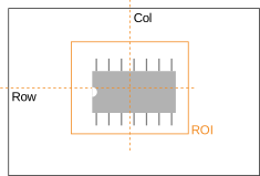 |
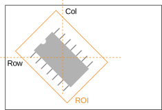 |
| Search image | 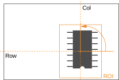 |
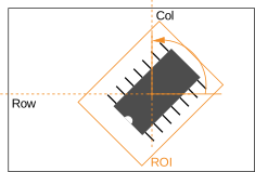 |
The center of the ROI (with image coordinates \(Row\) and \(Col\)) acts as the default point of reference.
In the template image, the orientation is always 0.
Display the Matches🔗
In many cases, especially during the development of a matching application, it is useful to display the matching results in the search image. This can be realized by different means. If the model is represented by a contour, we recommend to overlay the XLD contour on the search image, because XLD contours can be transformed more precisely and quickly than regions. Additionally, by displaying the contour of the model not only the position and orientation of the found model instance but also the deviation from the model’s shape can be visualized.
If no contour is available, we recommend to overlay the ROI that was used to create the model on the search image. In some cases, the additional visualization of points is suitable.
To demonstrate accessing and transforming a contour the example program %HALCONEXAMPLES%\hdevelop\Matching\Correlation-Based\ncc_matching_workflow.hdev, which uses of a correlation-based matching, is shown.
Step 1: Access the XLD contour containing the model
The XLD version of the model is accessed.
get_ncc_model_region (ModelRegion, ModelID[Index])
gen_contour_region_xld (ModelRegion, ModelContours, 'border_holes'
Step 2: Determine the affine transformation
A visualization is only reasonable if the matching was successful.
Thus, the results of the matching are checked.
If the matching failed, the operator find_ncc_model returns empty tuples in parameters like Row.
If the matching was successful, the corresponding affine transformation can be constructed.
hom_mat2d_identity (HomMat2DIdentity)
hom_mat2d_rotate (HomMat2DIdentity, Angle[Match], 0, 0, HomMat2DRotate)
hom_mat2d_translate (HomMat2DRotate, Row[Match], Column[Match], HomMat2DTranslate)
Note that also the transformation matrix can be constructed. Doing so, remember that the initial XLD contour of the model is located at the origin of the image and not at the position of the model in the reference image.
Step 3: Transform the XLD
Now, the transformation is applied to the XLD contour of the model using the operator affine_trans_contour_xld and the transformed contour is displayed.
affine_trans_contour_xld (ModelContours, ContoursAffinTrans, HomMat2DTranslate)
dev_display (ContoursAffinTrans)
The general procedure for the projection of a contour or a region is the same.
The main difference between the projection of a contour and the projection of a region regards the initial position of the contour or region.
The initial position of the contour or region always describes the “relative” position of the point of reference, that is, its distance to the default point of reference.
The default position of the point of reference is 0,0, that is, it is the origin of the image and not the position of the model in the reference image.
But depending on the structure that has to be transformed, the “relative” position can change.
Whereas the XLD contour of a shape model is derived from the model and thus its point of reference is also the point of reference of the model, a region naturally was defined before the model was created.
Thus, its point of reference describes the position of the model in the reference image instead of the point of reference of the later created model.
That is, instead of 0,0, the values obtained by the operator area_center for the respective region have to be passed as the first two parameters to vector_angle_to_rigid.
Furthermore, if you have changed the reference point of a model, the values to insert as initial position change in the following way.
If you query an XLD contour from a model after changing the point of reference, nothing changes.
The initial position still is 0,0, only another part of the model serves as point of reference.
If you change the point of reference after querying the XLD contour or if you want to transform a region, which is naturally also accessed before changing the point of reference, you have to add the values of the initial point of reference to the values of the new point of reference.
Align ROIs for other inspection tasks🔗
The results of matching can be used to align ROIs for other image processing steps. That is, to position them relative to the image part acting as the model. This method is suitable, for example, if the object to be inspected is allowed to move or if multiple instances of the object are to be inspected at once.
The example program %HALCONEXAMPLES%\solution_guide\matching\align_measurements.hdev uses shape-based matching to inspect multiple razor blades by measuring the width and the distance of their “teeth”.
First, a shape model is created that will be used later to align the measurement ROIs. shows the model ROI for the shape model, which consists of two united regions, and shows the corresponding shape model.
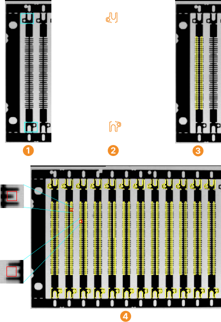
ROIs for the model
Model
Measuring ROIs
Inspection results with zoomed faults
Then, the inspection task is realized with the following steps:
Step 1: Position the measurement ROIs for the model blade
Two rectangular measurement ROIs are generated with gen_rectangle2 so that they are placed over the teeth of the razor blade that acts as the model (see
).
Rect1Row := 244
Rect1Col := 73
DistColRect1Rect2 := 17
Rect2Row := Rect1Row
Rect2Col := Rect1Col + DistColRect1Rect2
RectPhi := rad(90)
RectLength1 := 122
RectLength2 := 2
gen_rectangle2 (MeasureROI1, Rect1Row, Rect1Col, RectPhi, RectLength1, RectLength2)
gen_rectangle2 (MeasureROI2, Rect2Row, Rect2Col, RectPhi, RectLength1, RectLength2)
To be able to transform them later along with the XLD contour of the model, they are moved with move_region to lie on the XLD model, whose point of reference is the origin of the image (see Table 2, left), which is queried with area_center.
Note that before moving the regions the clipping must be switched off, otherwise the region parts that are moved “outside” the image are clipped.
The distances between the center of the model ROI and the centers of the rectangular measure ROIs define the new reference positions for the measure ROIs (see Table 2, right).
area_center (ModelROI, Area, CenterROIRow, CenterROIColumn)
get_system ('clip_region', OriginalClipRegion)
set_system ('clip_region', 'false')
move_region (MeasureROI1, MeasureROI1Ref, -CenterROIRow, -CenterROIColumn)
move_region (MeasureROI2, MeasureROI2Ref, -CenterROIRow, -CenterROIColumn)
set_system ('clip_region', OriginalClipRegion)
DistRect1CenterRow := Rect1Row - CenterROIRow
DistRect1CenterCol := Rect1Col - CenterROIColumn
DistRect2CenterRow := Rect2Row - CenterROIRow
DistRect2CenterCol := Rect2Col - CenterROIColumn
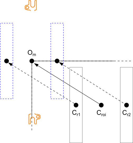 |
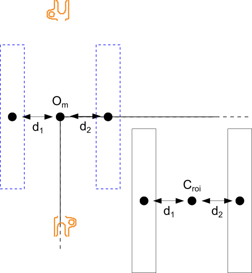 |
|
|---|---|---|
| Move the measure ROIs to lie on the XLD model | Determine the new reference positions for the measure ROIs by their distance to the model |
\(O_m\): model origin
\(C_{r1}\): center of rectangle 1
\(C_{r2}\): center of rectangle 2
\(C_{roi}\): center of ROI
\(d_1\): distance 1
\(d_2\): distance 2
Step 2: Find all razor blades
Now, all instances of the shape model are searched for in the search image using find_generic_shape_model.
Step 3: Determine the affine transformation
For each instance, that is, for each found razor blade, the transformation between the model and the found model instance is calculated with vector_angle_to_rigid and applied to the XLD model with affine_trans_contour_xld so that it lies over the found model instance in the search image.
for I := 0 to NumMatchResult - 1 by 1
    get_generic_shape_model_result (MatchResultID, Indices[I], 'row', RowCheck)
    get_generic_shape_model_result (MatchResultID, Indices[I], 'column', ColumnCheck)
    get_generic_shape_model_result (MatchResultID, Indices[I], 'angle', AngleCheck)
    vector_angle_to_rigid (0, 0, 0, RowCheck, ColumnCheck, AngleCheck, MovementOfObject)
    affine_trans_contour_xld (ModelContours, ModelAtNewPosition, MovementOfObject)
Step 4: Create measurement objects at the corresponding positions
Then, affine_trans_pixel is applied to calculate the corresponding positions of the measure ROIs, at which the measure objects are created.
affine_trans_pixel (MovementOfObject, DistRect1CenterRow, DistRect1CenterCol, Rect1RowCheck, Rect1ColCheck)
affine_trans_pixel (MovementOfObject, DistRect2CenterRow, DistRect2CenterCol, Rect2RowCheck, Rect2ColCheck)
RectPhiCheck := RectPhi + AngleCheck
gen_measure_rectangle2 (Rect1RowCheck, Rect1ColCheck, RectPhiCheck, RectLength1, RectLength2, Width, Height, 'bilinear', MeasureHandle1)
gen_measure_rectangle2 (Rect2RowCheck, Rect2ColCheck, RectPhiCheck, RectLength1, RectLength2, Width, Height, 'bilinear', MeasureHandle2)
Note that you must use the operator affine_trans_pixel and not affine_trans_point_2d, because the latter uses a different coordinate system.
In particular, it uses the standard image coordinate system for which a position corresponds to the center of a pixel (see Figure 2, right).
In contrast, the operators affine_trans_pixel, affine_trans_contour_xld, affine_trans_region, and affine_trans_image use the coordinate system depicted in Figure 2 (left).
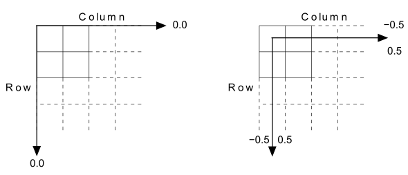
affine_trans_pixel (left) and standard image coordinate system (right). In the example application, the individual razor blades are only translated but not rotated relative to the model position.
Thus, instead of applying the full affine transformation to the measure ROIs and then creating new measure objects, you can use the operator translate_measure to translate the measure objects themselves.
The example program contains the corresponding code.
You can switch between the two methods by modifying a variable at the top of the program.
Step 5: Measure the width and the distance of the “teeth”
Now, the actual measurements are performed using the operator measure_pairs.
measure_pairs (SearchImage, MeasureHandle1, 2, 25, 'negative', 'all', RowEdge11, ColEdge11, Amp11, RowEdge21, ColEdge21, Amp21, Width1, Distance1)
measure_pairs (SearchImage, MeasureHandle2, 2, 25, 'negative', 'all', RowEdge12, ColEdge12, Amp12, RowEdge22, ColEdge22, Amp22, Width2, Distance2)
Step 6: Inspect the measurements
Finally, the measurements are inspected. If a tooth is too short or missing completely, no edges are extracted at this point resulting in an incorrect number of extracted edge pairs. In this case, the faulty position can be determined by checking the distance of the teeth. Figure 1 shows the inspection results for the example.
NumberTeeth1 := |Width1|
if (NumberTeeth1 < 37)
    for J := 0 to NumberTeeth1 - 2 by 1
        if (Distance1[J] > 4.0)
            RowFault := round(0.5 * (RowEdge11[J + 1] + RowEdge21[J]))
            ColFault := round(0.5 * (ColEdge11[J + 1] + ColEdge21[J]))
            disp_rectangle2 (WindowHandle, RowFault, ColFault, 0, 4, 4)
Please note that the example program is not able to display the fault if it occurs at the first or the last tooth.
Align the Search Results🔗
You can also determine the inverse transformation which transforms objects from the search image back into the reference image.
With this transformation, you can align the search image (or parts of it), that is, transform it such that the matched object is positioned as it was in the reference image. This method is useful if the following image processing step is not invariant against rotation, for example, OCR or the variation model.
Note that by alignment the image is only rotated and translated. To remove perspective or lens distortions, for example, if the camera observes the scene under an oblique angle, you must rectify the image first.
Inverse transformation🔗
The inverse transformation can be determined and applied in a few steps.
The task of the example program %HALCONEXAMPLES%\solution_guide\matching\rectify_results.hdev, is to extract the serial number on CD covers (see Figure 3.
The matching is realized using a shape-based matching.
Step 1: Calculate the inverse transformation
As a first step the transformation matrix is calculated based on the absolute coordinates of the point of reference, because the results have to be transformed such that they appear as in the reference image.
get_generic_shape_model_result (MatchResultID, 'best', 'row', RowMatch)
get_generic_shape_model_result (MatchResultID, 'best', 'column', ColumnMatch)
get_generic_shape_model_result (MatchResultID, 'best', 'angle', AngleMatch)
vector_angle_to_rigid (CenterModelROIRow, CenterModelROIColumn, 0, RowMatch, ColumnMatch, AngleMatch, MovementOfObject)
Note, this transformation matrix can also be created in different ways, for example, by operating the model transformation matrix on the original center of RoI.
You can invert a transformation easily using the operator hom_mat2d_invert.
Step 2: Rectify the search image
The inverse transformation is applied to the search image using the operator affine_trans_image.
Figure 3
shows the resulting rectified image of a different CD.
Undefined pixels are marked in gray.
affine_trans_image (SearchImage, RectifiedSearchImage, InverseMovementOfObject, 'constant', 'false')
Step 3: Extract the numbers
The serial number is positioned correctly within the original ROI and can be extracted by blob analysis without problems. Figure 3 shows the result, which could then, for example, be used as the input for OCR.
reduce_domain (RectifiedSearchImage, NumberROI, RectifiedNumberROIImage)
threshold (RectifiedNumberROIImage, Numbers, 0, 128)
connection (Numbers, IndividualNumbers)
Unfortunately, the operator affine_trans_image transforms the full image even if its domain was restricted with the operator reduce_domain.
In a time-critical application it may therefore be necessary to crop the search image before transforming it.
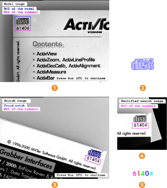
ROIs for the model and for the number extraction
model
found model and number ROI at matched position
rectified search image (only relevant part shown)
extracted numbers
Image cropping🔗
In the following, the steps needed for the image cropping are described. Additionally, they are visualized in Figure 4.
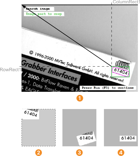
smallest image part containing the ROI
cropped search image
result of the rectification
rectified image reduced to the original number ROI
Step 1: Crop the search image
First, the smallest axis-parallel rectangle surrounding the transformed number ROI is computed using the operator smallest_rectangle1.
Then, the search image is cropped to this part with crop_rectangle1.
Figure 4
shows the resulting image overlaid on a gray rectangle to facilitate the comparison with the subsequent images.
affine_trans_region (NumberROI, NumberROIAtNewPosition, MovementOfObject, 'nearest_neighbor')
smallest_rectangle1 (NumberROIAtNewPosition, RowRect1, ColumnRect1, RowRect2, ColumnRect2)
crop_rectangle1 (SearchImage, CroppedSearchImage, RowRect1, ColumnRect1, RowRect2, ColumnRect2)
Step 2: Create an extended affine transformation
In fact, the cropping can be interpreted as an additional affine transformation, in particular, as a translation by the negated coordinates of the upper left corner of the cropping rectangle (see Figure 4
).
We therefore add this transformation to the transformation that describes the movement of the object using the operator hom_mat2d_translate.
Then, we invert this extended transformation with the operator hom_mat2d_invert.
hom_mat2d_translate (MovementOfObject, -RowRect1, -ColumnRect1, MoveAndCrop)
hom_mat2d_invert (MoveAndCrop, InverseMoveAndCrop)
Step 3: Transform the cropped image
Using the inverted extended transformation, the cropped image can easily be rectified with the operator affine_trans_image (Figure 4
) and then be reduced to the original number ROI (Figure 4
) in order to extract the numbers.
affine_trans_image (CroppedSearchImage, RectifiedROIImage, InverseMoveAndCrop, 'constant', 'true')
reduce_domain (RectifiedROIImage, NumberROI, RectifiedNumberROIImage)
Visualizing matches and perform transformations using a 2D homography When applying one of the uncalibrated perspective matching approaches, in contrast to the pure 2D matching approaches no positions, orientations, and scales but projective transformation matrices are returned.🔗
These can be used to apply a projective transformation, for example, to visualize the matching result by overlaying a structure of the reference image on the match in the search image. Note that different HALCON structures like pixels, regions, images, or XLD contours can be transformed that way.
Depending on the selected matching approach, typically different structures are transformed. For the uncalibrated perspective deformable matching, for example, the model contour is transformed to visualize the match, whereas for the uncalibrated descriptor-based matching the region that was used to create the model may be transformed and visualized.
An example for a projective transformation in the context of an uncalibrated perspective deformable matching is given in the example program %HALCONEXAMPLES%\hdevelop\Applications\Traffic-Monitoring\detect_road_signs.hdev.
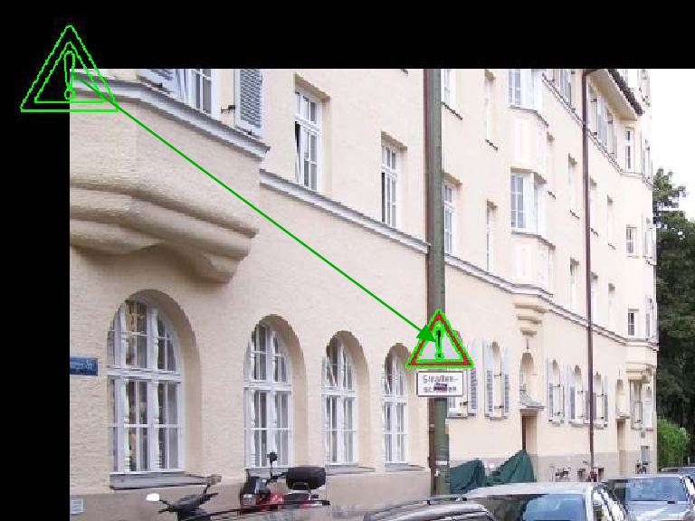
Step 1: Find the perspective deformable model
There, the model of a road sign is searched in an image using find_planar_uncalib_deformable_model, which returns the projective transformation matrix HomMat2D.
find_planar_uncalib_deformable_model (ImageChannel, Models[Index2], 0, 0, ScaleRMin[Index2], ScaleRMax[Index2], ScaleCMin[Index2], ScaleCMax[Index2], 0.85, 1, 0, 2, 0.4, [], [], HomMat2D, Score)
Step 2: Transform the model contours
After the matching, the model contours are queried from the model with get_deformable_model_contours.
The returned contours are by default positioned at the origin of the reference image.
Thus, to visualize them at the position of the match, the contour must be transformed using the returned projective transformation matrix.
This transformation is applied with projective_trans_contour_xld.
get_deformable_model_contours (ModelContours, Models[Index2], 1)
projective_trans_contour_xld (ModelContours, ContoursProjTrans, HomMat2D)
dev_display (ContoursProjTrans)
An example for a projective transformation in the context of an uncalibrated descriptor-based matching is the example program %HALCONEXAMPLES%\hdevelop\Applications\Object-Recognition-2D\detect_brochure_pages.hdev (see Figure 6).
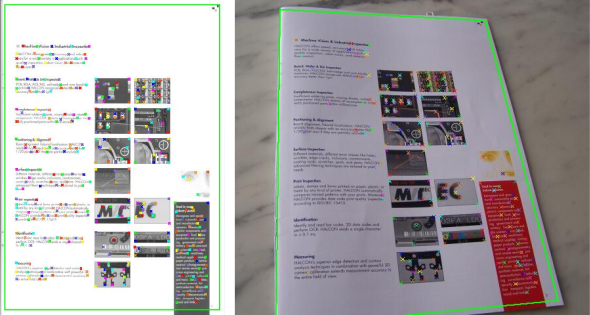
Step 1: Find the descriptor model
There, the projective transformation matrix HomMat2D is returned by find_uncalib_descriptor_model.
find_uncalib_descriptor_model (ImageGray, ModelIDs[Index2], 'threshold', 600, ['min_score_descr', 'guided_matching'], [0.003, 'on'], 0.25, 1, 'num_points', HomMat2D, Score)
Step 2: Access and visualize the interest points
The interest points are queried with get_descriptor_model_points.
In contrast to the contours of a perspective deformable model, which can only be queried for the model, the points of the descriptor model can also be queried for the specific match (Set set to 'search').
Thus, they do not have to be transformed anymore.
get_descriptor_model_points (ModelIDs[Index2], 'search', 0, Row, Col)
gen_cross_contour_xld (Cross, Row, Col, 6, 0.785398)
Step 3: Transform the model region and its corner points
Projective transformations can be used if, for example, the transformed region that was used for the creation of the model should be visualized for the match as well or if the transformed corner points of the region are needed to check the angle between edges of the region.
projective_trans_region (Rectangle, TransRegion, HomMat2D, 'bilinear')
projective_trans_pixel (HomMat2D, RowRoi, ColRoi, RowTrans, ColTrans)
angle_ll (RowTrans[2], ColTrans[2], RowTrans[1], ColTrans[1], RowTrans[1], ColTrans[1], RowTrans[0], ColTrans[0], Angle)
Angle := deg(Angle)
if (Angle > 70 and Angle < 110)
    dev_display (TransRegion)
    dev_display (Cross)
endif