Uncalibrated Image Mosaicking🔗
If you need an image of a large object, but the field of view of the camera does not allow to cover the entire object with the desired resolution, you can use image mosaicking to generate a large image of the entire object from a sequence of overlapping images of parts of the object.
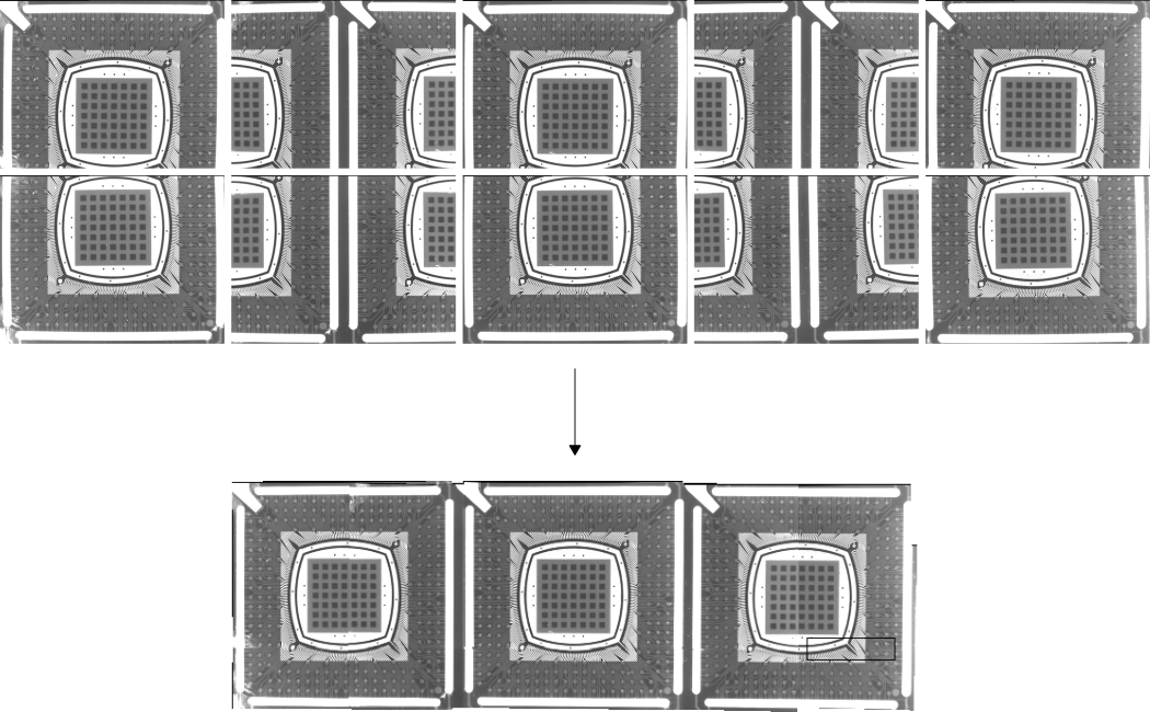
An example for such an application is given in Figure 1. On the left side, six separate images are displayed stacked upon each other. On the right side, the mosaic image generated from the six separate images is shown. Note that the folds visible in the image do not result from the mosaicking. They are due to some degradations on the PCB, which can be seen already in the separate images.
Example for a mosaicking application.
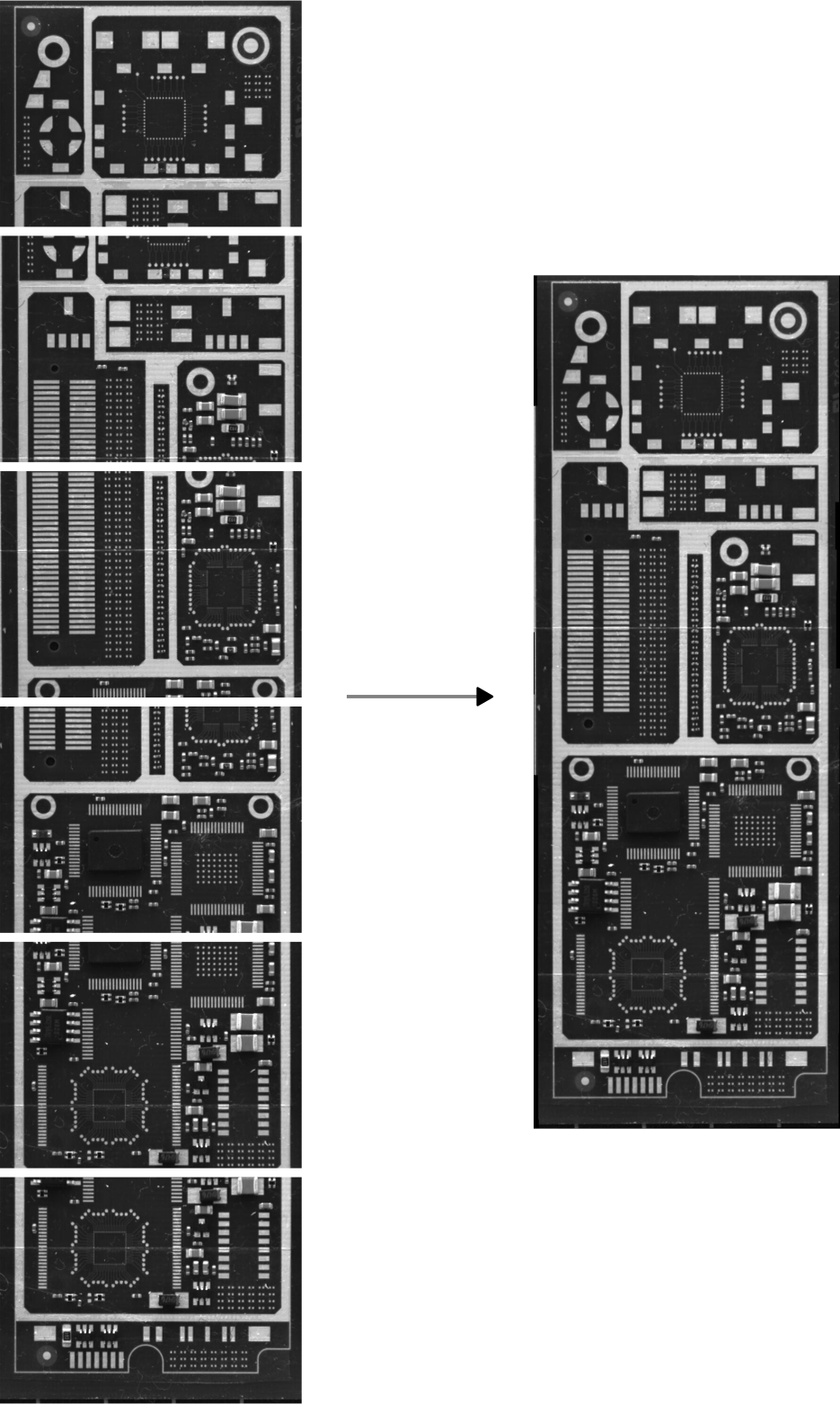
The mosaicking approach described in this section is designed for applications where it is not necessary to achieve the high-precision mosaic images. The advantages compared to this approach are that no camera calibration is necessary and that the individual images can be arranged automatically.
The example program %HALCONEXAMPLES%\solution_guide\3d_vision\mosaicking.hdev generates a mosaic image from a sequence of images.
First, the images are read from file and collected in one tuple.
gen_empty_obj (Images)
for J := 1 to 10 by 1
    read_image (Image, ImgPath + ImgName + J$'02')
    concat_obj (Images, Image, Images)
endforFrom := [1, 2, 3, 4, 6, 7, 8, 9, 3]
To := [2, 3, 4, 5, 7, 8, 9, 10, 8]Now, characteristic points must be extracted from the images, which are then used for the matching between the image pairs. The resulting projective transformation matrices must be accumulated.
Num := |From|
ProjMatrices := []
for J := 0 to Num - 1 by 1
    F := From[J]
    T := To[J]
    select_obj (Images, ImageFrom, F)
    select_obj (Images, ImageTo, T)
    points_harris (ImageFrom, SigmaGrad, SigmaSmooth, Alpha, Threshold, RowFromAll, ColumnFromAll)
    points_harris (ImageTo, SigmaGrad, SigmaSmooth, Alpha, Threshold, RowToAll, ColumnToAll)
    proj_match_points_ransac (ImageFrom, ImageTo, RowFromAll, ColumnFromAll, RowToAll, ColumnToAll, 'sad', MaskSize, RowMove, ColumnMove, RowTolerance, ColumnTolerance, Rotation, MatchThreshold, 'gold_standard', DistanceThreshold, RandSeed, ProjMatrix, Points1, Points2)
    ProjMatrices := [ProjMatrices,ProjMatrix]
    disp_message (WindowHandle1, 'Point matches', 'window', 12, 12, 'black', 'true')
Finally, the image mosaic can be generated.
gen_projective_mosaic (Images, MosaicImage, StartImage, From, To, ProjMatrices, StackingOrder, 'false', MosaicMatrices2D)Note that image mosaicking is a tool for a quick and easy generation of large images from several overlapping images. For this task, it is not necessary to calibrate the camera. If you need a high-precision image mosaic, you should use calibrated mosaicking.
In the following sections, the individual steps for the generation of a mosaic image are described.
Rules for taking images for a mosaic image🔗
The following rules for the acquisition of the separate images should be considered:
- The images must overlap each other.
- The overlapping area of the images must be textured in order to allow the automatic matching process to identify identical points in the images. The lack of texture in some overlapping areas may be overcome by an appropriate definition of the image pairs. If the whole object shows little texture, the overlapping areas should be chosen larger.
- Overlapping images must have approximately the same scale. In general, the scale differences should not exceed 5-10%.
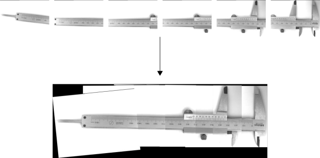
- The images should be radiometrically similar, at least in the overlapping areas, as no radiometric adaption of the images is carried out. Otherwise, i.e., if the brightness differs heavily between neighboring images, the seams between them will be clearly visible as can be seen in Figure 2.
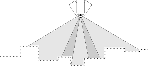
The images are mapped onto a common image plane using a projective transformation. Therefore, to generate a geometrically accurate image mosaic from images of non-flat objects, the separate images must be acquired from approximately the same point of view, i.e., the camera can only be rotated around its optical center (see Figure 3).
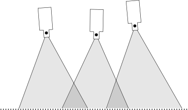
When dealing with flat objects, it is possible to acquire the images from arbitrary positions and with arbitrary orientations if the scale difference between the overlapping images is not too large (Figure 4).
The lens distortions of the images are not compensated by the mosaicking process. Therefore, if lens distortions are present in the images, they cannot be mosaicked with high accuracy, i.e., small distortions at the seams between neighboring images cannot be prevented (see Table 1). To eliminate this effect, the lens distortions can be compensated before starting the mosaicking process (see Calibration > Rectification).
If processing time is an issue, it is advisable to acquire the images in the same orientation, i.e., neither the camera nor the object should be rotated around the optical axis, too much. Then, the rotation range can be restricted for the matching process.
Defining overlapping image pairs🔗
As shown in the introductory example, it is necessary to define the overlapping image pairs between which the transformation is to be determined. The successive matching process will be carried out for these image pairs only.
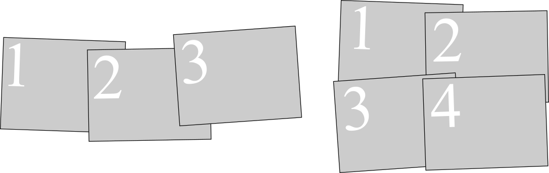
Figure 5 shows two configurations of separate images.
For the left configuration, the definition of the image pairs is simply (1,2) and (2,3), which can be defined in as:
From := [1,2]
To := [2,3]
In any case, it is important to ensure that each image must be ‘connected’ to all the other images. For example, for the right configuration of Figure 5, it is not possible to define the image pairs as (1,2) and (3,4), only, because images 1 and 2 would not be connected to images 3 and 4. In this case, it would, e.g., be possible to define the three image pairs (1,2), (1,3), and (2,4).
From := [1,1,2]
To := [2,3,4]
Assuming there is no texture in the overlapping area of image two and four, the matching could be carried out between images three and four instead.
From := [1,1,3]
To := [2,3,4]
If a larger number of separate images are mosaicked, or, e.g., an image configuration similar to the one displayed in Figure 6, where there are elongated rows of overlapping images, it is important to thoroughly arrange the image pair configuration. Otherwise it is possible that some images do not fit together precisely. This happens since the transformations between the images cannot be determined with perfect accuracy because of very small errors in the point coordinates due to noise. These errors are propagated from one image to the other.
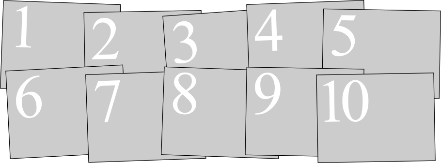
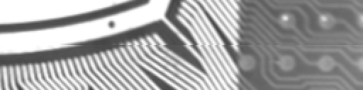
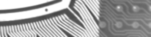
Figure 7 shows such an image sequence of ten images of a BGA and the resulting mosaic image. Table 1 shows a cut-out of that mosaic image. It depicts the seam between image 5 and image 10 for two image pair configurations, using the original images and the images where the lens distortions have been eliminated, respectively. The position of the cut-out is indicated in Figure 7 by a rectangle.
| with lens distortions | lens distortions eliminated | |
|---|---|---|
| unfavorable configuration | 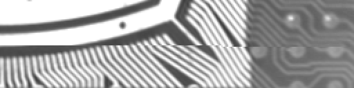 |
 |
| good configuration | 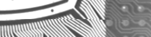 |
 |
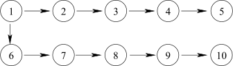
First, the matching has been carried out in the two image rows separately and the two rows are connected via image pair 1 → 6.
From := [1,2,3,4,6,7,8,9,1]
To := [2,3,4,5,7,8,9,10,6]
In this configuration the two neighboring images 5 and 10 are connected along a relatively long path. To improve the geometrical accuracy of the image mosaic, the connections between the two image rows could be established by the image pair (3,8), as visualized in Table 2.
| unfavorable configuration | good configuration |
|---|---|
 |
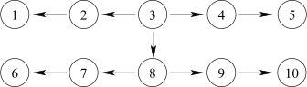 |
This can be achieved by defining the image pairs as follows.
From := [1,2,3,4,6,7,8,9,3]
To := [2,3,4,5,7,8,9,10,8]
As can be seen in Table 1, now the neighboring images fit better.
Recapitulating, there are three basic rules for the arrangement of the image pairs:
Take care that
- each image is connected to all the other images.
- the path along which neighboring images are connected is not too long.
- the overlapping areas of image pairs are large enough and contain enough texture to ensure a proper matching.
In principle, it is also possible to define more image pairs than required (number of images minus one). However, then it cannot be controlled which pairs are actually used. Therefore, we do not recommend this approach.
Detecting characteristic points🔗
HALCON provides you with various operators for the extraction of characteristic points (interest points). The most important of these operators are
points_foerstnerpoints_harrisandpoints_harris_binomialpoints_lepetitpoints_sojkasaddle_points_sub_pix
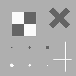
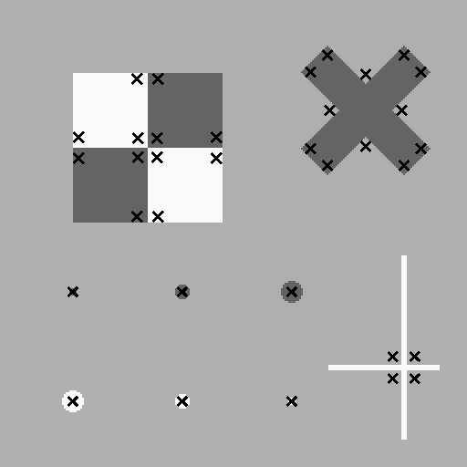
All of these operators can determine the coordinates of interest points with subpixel accuracy. Below, a test image together with typical results of these interest operators is displayed.
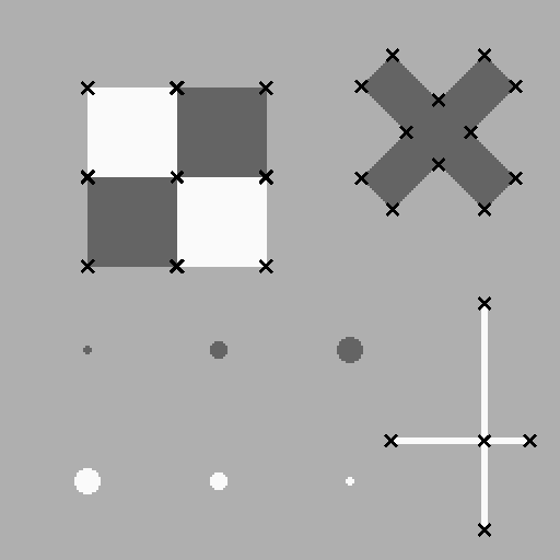
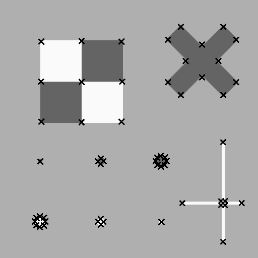
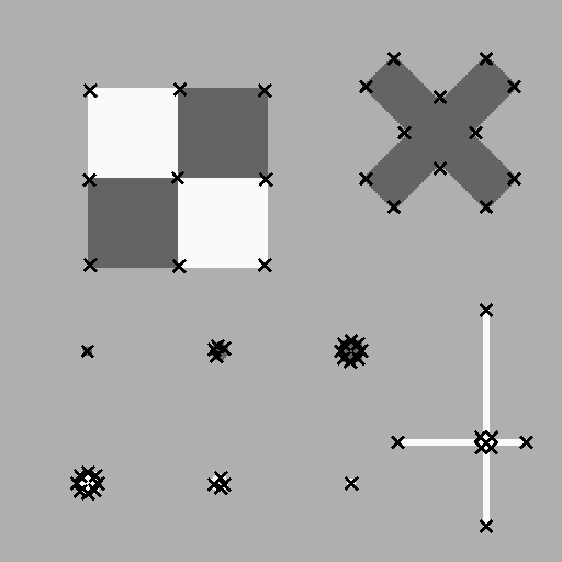
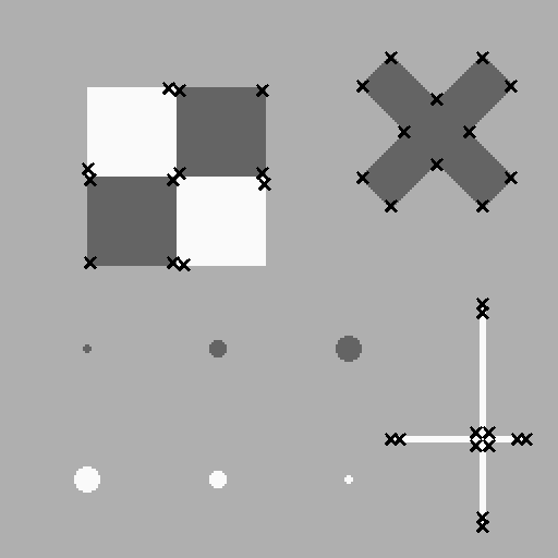
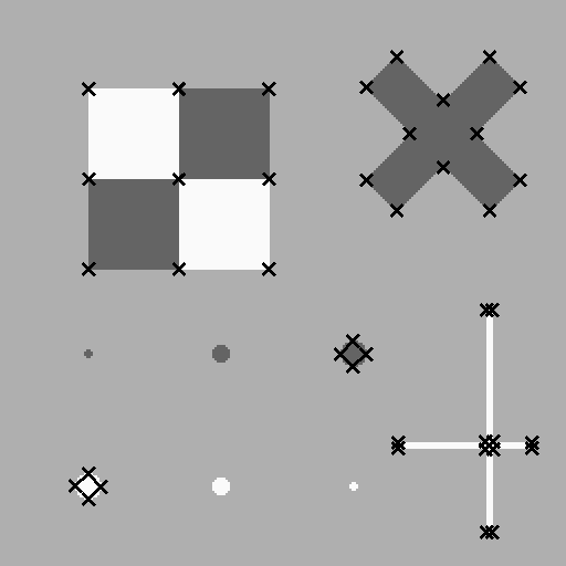
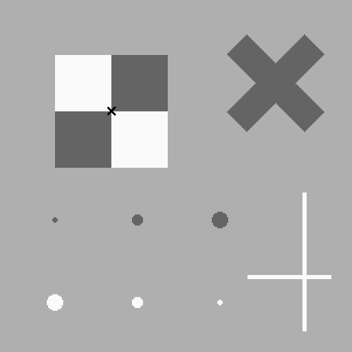
The operator points_foerstner classifies the interest points into two categories: junction-like features and area-like features.
The results are very reproducible even in images taken from a different point of view.
Therefore, it is very well suited for the extraction of points for the subsequent matching.
It is very accurate but computationally the most expensive operator out of the interest operators presented in this section.
The results of the operator points_harris are very reproducible, too.
Admittedly, the points extracted by the operator points_harris are sometimes not meaningful to a human, e.g., they often lie slightly beside a corner or an eye-catching image structure.
Nevertheless, it is faster than the operator points_foerstner.
The operator points_harris_binomial detects points of interest using the binomial approximation of the points_harris operator.
It is therefore faster than points_harris.
The operator points_lepetit extracts points of interest like corners or blob-like structures from the image.
This operator can especially be used for very fast interest point extraction.
It is the fastest out of the six operators presented in this section.
The operator points_sojka is specialized in the extraction of corner points.
The operator saddle_points_sub_pix is designed especially for the extraction of saddle points, i.e., points whose image intensity is minimal along one direction and maximal along a different direction.
The number of interest points influence the execution time and the result of the subsequent matching process. The more interest points are used, the longer the matching takes. If too few points are used the probability of an erroneous result increases.
In most cases, the default parameters of the interest operators need not be changed.
Only if too many or too few interest points are found adaptations of the parameters might be necessary.
For a description of the parameters, please refer to the respective pages of the Reference Manual (points_foerstner, points_harris, points_harris_binomial, points_lepetit, points_sojka, saddle_points_sub_pix).
Matching characteristic points in overlapping areas🔗
The most demanding task during the generation of an image mosaic is the matching process.
The operator proj_match_points_ransac is able to perform the matching even if the two images are shifted and rotated arbitrarily.
proj_match_points_ransac (ImageFrom, ImageTo, RowFromAll, ColumnFromAll, RowToAll, ColumnToAll, 'sad', MaskSize, RowMove, ColumnMove, RowTolerance, ColumnTolerance, Rotation, MatchThreshold, 'gold_standard', DistanceThreshold, RandSeed, ProjMatrix, Points1, Points2)The only requirement is that the images should have approximately the same scale. If information about shift and rotation is available it can be used to restrict the search space, which speeds up the matching process and makes it more robust.
In case the matching fails, ensure that there are enough characteristic points and that the search space and the maximum rotation are defined appropriately.
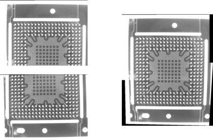
If the images that should be mosaicked contain repetitive patterns, like the two images of a BGA shown in Figure 8 (left), it may happen that the matching does not work correctly.
In the resulting erroneous mosaic image, the separate images may not fit together or may be heavily distorted.
To achieve a correct matching result for such images, it is important to provide initial values for the shift between the images with the parameters RowMove and ColMove.
In addition, the search space should be restricted to an area that contains only one instance of the repetitive pattern, i.e., the values of the parameters RowTolerance and ColTolerance should be chosen smaller than the distance between the instances of the repetitive pattern.
With this, it is possible to obtain proper mosaic images, even for objects like BGAs (see Figure 8, right).
For a detailed description of the other parameters, please refer to the operator reference of (proj_match_points_ransac).
The results of the operator proj_match_points_ransac are the projective transformation matrix and the two tuples Points1 and Points2 that contain the indices of the matched input points from the two images.
The projective transformation matrices resulting from the matching between the image pairs must be accumulated.
ProjMatrices := [ProjMatrices,ProjMatrix]Alternatively, if it is known that the mapping between the images is a rigid 2D transformation, the operator proj_match_points_ransac can be used to determine the point correspondences only, since it returns the indices of the corresponding points in the tuples Points1 and Points2.
With this, the corresponding point coordinates can be selected.
RowFrom := subset(RowFromAll,Points1)
ColumnFrom := subset(ColumnFromAll,Points1)
RowTo := subset(RowToAll,Points2)
ColumnTo := subset(ColumnToAll,Points2)
Then, the rigid transformation between the image pair can be determined with the operator vector_to_rigid.
Note that we have to add 0.5 to the coordinates to make the extracted pixel positions fit the coordinate system that is used by the operator gen_projective_mosaic.
vector_to_rigid (RowFrom + 0.5, ColumnFrom + 0.5, RowTo + 0.5, ColumnTo + 0.5, HomMat2D)Because gen_projective_mosaic expects a 3\(\times\)3 transformation matrix, but vector_to_rigid returns a 2\(\times\)3 matrix, we have to add the last row [0,0,1] to the transformation matrix before we can accumulate it.
ProjMatrix := [HomMat2D,0, 0, 1]
ProjMatrices := [ProjMatrices,ProjMatrix]
Furthermore, the operator proj_match_points_ransac_guided is available.
Like proj_match_points_ransac, it can be used to calculate the projective transformation matrix between two images by finding correspondences between points.
But in contrast to proj_match_points_ransac, it is based on a known approximation of the projective transformation matrix.
Thus, it can be used, for example, to speed up the matching of very large images by implementing an image-pyramid-based projective matching algorithm.
The example program %HALCONEXAMPLES%\hdevelop\Tools\Mosaicking\mosaicking_pyramid.hdev shows how to implement the image-pyramid-based approach and compares the runtime
Generating the mosaic image🔗
Once the transformations between the image pairs are known the mosaic image can be generated with the operator gen_projective_mosaic.
gen_projective_mosaic (Images, MosaicImage, StartImage, From, To, ProjMatrices, StackingOrder, 'false', MosaicMatrices2D)It requires the images to be given in a tuple.
All images are projected into the image plane of a so-called start image.
The start image can be defined by its position in the image tuple (starting with 1) with the parameter StartImage.
Additionally, the image pairs must be specified together with the corresponding transformation matrices.
The order in which the images are added to the mosaic image can be specified with the parameter StackingOrder.
The first index in this array will end up at the bottom of the image stack while the last one will be on top.
If 'default' is given instead of an array of integers, the canonical order (the order in which the images are given) will be used.
If the domains of the images should be transformed as well, the parameter TransformRegion must be set to 'true'.
The output parameter MosaicMatrices2D contains the projective 3\(\times\)3 transformation matrices for the mapping of the separate images into the mosaic image.
These matrices can, e.g., be used to transform features extracted from the separate images into the mosaic image by using the operators projective_trans_pixel, projective_trans_region, projective_trans_contour_xld, or projective_trans_image.
Bundle adjusted mosaicking🔗
It is also possible to generate the mosaic based on the matching results of all overlapping image pairs.
The transformation matrices between the images are then determined together within one bundle adjustment.
For this, the operators bundle_adjust_mosaic and gen_bundle_adjusted_mosaic are used.
The main advantage of the bundle adjusted mosaicking compared with the mosaicking based on single image pairs is that the bundle adjustment determines the geometry of the mosaic as robustly as possible. Typically, this leads to more accurate results. Another advantage is that there is no need to figure out a good pair configuration, you simply pass the matching results of all overlapping image pairs. What is more, it is possible to define the class of transformations that is used for the transformation between the individual images. A disadvantage of the bundle adjusted mosaicking is that it takes more time to perform the matching between all overlapping image pairs instead of just using a subset. Furthermore, if the matching between two images was erroneous, sometimes the respective image pair is difficult to find in the set of all image pairs.
With this, it is obvious that the bundle adjustment is worthwhile if there are multiple overlaps between the images, i.e., if there are more than \(n-1\) overlapping image pairs, with \(n\) being the number of images. Another reason for using the bundle adjusted mosaicking is the possibility to define the class of transformations.
The example program %HALCONEXAMPLES%\solution_guide\3d_vision\bundle_adjusted_mosaicking.hdev shows how to generate the bundle adjusted mosaic from the ten images of the BGA displayed in reffig{mosaicking:pairs:configuration_ten_images}.
The design of the program is very similar to that of the example program %HALCONEXAMPLES%\solution_guide\3d_vision\mosaicking.hdev.
The main differences are that
- the matching is carried out between all overlapping images,
- in addition to the projective transformation matrices also the coordinates of the corresponding points must be accumulated, and
- the operator
gen_projective_mosaicis replaced with the operatorsbundle_adjust_mosaicandgen_bundle_adjusted_mosaic.
First, the matching is carried out between all overlapping image pairs, which can be defined as follows:
From := [1, 1, 1, 2, 2, 2, 2, 3, 3, 3, 3, 4, 4, 4, 4, 5, 5]
To := [6, 7, 2, 6, 7, 8, 3, 7, 8, 9, 4, 8, 9, 10, 5, 9, 10]
In addition to the accumulation of the projective transformation matrices, also the coordinates of the corresponding points as well as the number of corresponding points must be accumulated.
Rows1 := [Rows1,subset(RowFAll,Points1)]
Cols1 := [Cols1,subset(ColFAll,Points1)]
Rows2 := [Rows2,subset(RowTAll,Points2)]
Cols2 := [Cols2,subset(ColTAll,Points2)]
NumCorrespondences := [NumCorrespondences,|Points1|]
This data is needed by the operator bundle_adjust_mosaic, which determines the bundle adjusted transformation matrices.
bundle_adjust_mosaic (10, StartImage, From, To, ProjMatrices, Rows1, Cols1, Rows2, Cols2, NumCorrespondences, Transformation, MosaicMatrices2D, Rows, Cols, Error)The parameter Transformation defines the class of transformations that is used for the transformation between the individual images.
Possible values are 'projective', 'affine', 'similarity', and 'rigid'.
Thus, if you know, e.g., that the camera looks perpendicular onto a planar object and that the camera movement between the images is restricted to rotations and translations in the object plane, you can choose the transformation class 'rigid'.
If translations may also occur in the direction perpendicular to the object plane, you must use 'similarity' because this transformation class allows scale differences between the images.
If the camera looks tilted onto the object, the transformation class 'projective' must be used, which can be approximated by the transformation class 'affine'.
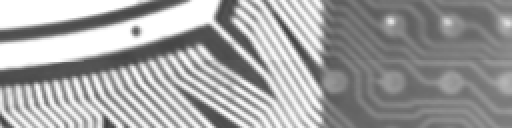
The tabbing below shows cut-outs of the resulting mosaic images.
They depict the seam between image 5 and image 10.
The mosaic images have been created using the images where the lens distortions have been eliminated.
The position of the cut-out within the whole mosaic image is indicated by the rectangle in Figure 6.
Finally, with the transformation matrices MosaicMatrices2D, which are determined by the operator bundle_adjust_mosaic, the mosaic can be generated with the operator gen_bundle_adjusted_mosaic.
gen_bundle_adjusted_mosaic (Images, MosaicImage, MosaicMatrices2D, StackingOrder, TransformRegion, TransMat2D)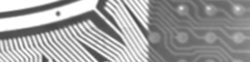
Spherical mosaicking🔗
The methods described in the previous sections arranged the images on a plane. As the name suggests, using spherical mosaicking you can arrange them on a sphere instead. Note that this method can only be used if the camera is only rotated around its optical center or zoomed. If the camera movement includes a translation or if the rotation is not performed exactly around the optical center, the resulting mosaic image will not be accurate and can therefore not be used for high-accuracy applications.
To create a spherical mosaic, you first perform the matching as described in the previous sections to determine the projective transformation matrices between the individual images.
This information is the input for the operator stationary_camera_self_calibration, which determines the internal camera parameters of the camera and the rotation matrices for each image.
Based on this information, the operator gen_spherical_mosaic then creates the mosaic image.
Please have a look at the example program %HALCONEXAMPLES%\hdevelop\Calibration\Self-Calibration\stationary_camera_self_calibration.hdev for more information about how to use these operators.
As an alternative, you can map the images on the six sides of a cube using gen_cube_map_mosaic.
Cube maps are especially useful in computer graphics.