Rectifying arbitrary distortions🔗
For many applications like OCR or bar code reading, distorted images must be rectified prior to the extraction of information. The distortions may be caused by the perspective projection and by the radial lens distortions as well as by the decentering lens distortions, a non-flat object surface, or by any other reason. In the first three cases, i.e., if the object surface is flat and the camera shows only radial or decentering distortions, the rectification can be carried out very precisely. For the remaining cases, a piecewise bilinear rectification can be carried out. In HALCON, this kind of rectification is called grid rectification.
The following example (%HALCONEXAMPLES%\hdevelop\Tools\Grid-Rectification\grid_rectification.hdev) shows how the grid rectification can be used to rectify the image of a cylindrically shaped object (Figure 1).
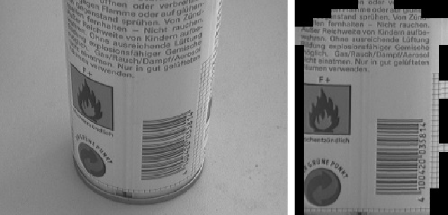
The main idea of the grid rectification is that the mapping for the rectification is determined from an image of the object, where the object is covered by a known pattern.
First, this pattern, which is called rectification grid, must be created with the operator create_rectification_grid.
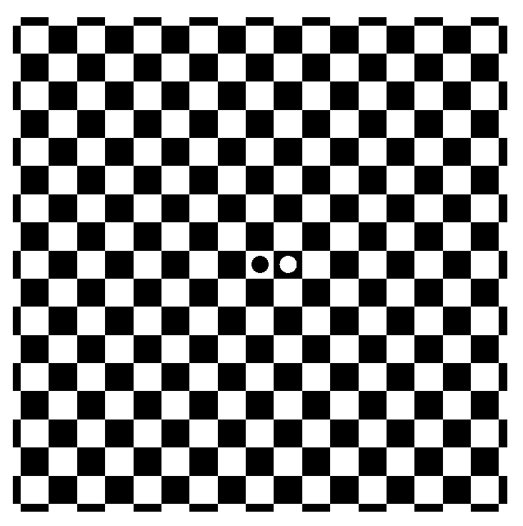
create_rectification_grid (WidthOfGrid, NumSquares, 'rectification_grid.ps')The resulting PostScript file must be printed. An example for such a rectification grid is shown in Figure 2.
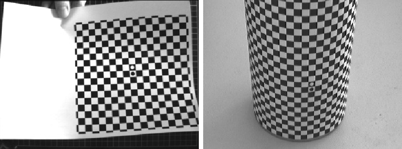
Now, the object must be wrapped with the rectification grid and an image of the wrapped object must be taken.
From this image, the mapping that describes the transformation from the distorted image into the rectified image can be derived. For this, first, the rectification grid must be extracted. Then, the rectification map is derived from the distorted grid. This can be achieved by the following lines of code:
find_rectification_grid (Image, GridRegion, MinContrast, Radius)
reduce_domain (Image, GridRegion, ImageReduced)
saddle_points_sub_pix (ImageReduced, 'facet', SigmaSaddlePoints, Threshold, Row, Col)
connect_grid_points (ImageReduced, ConnectingLines, Row, Col, SigmaConnectGridPoints, MaxDist)
gen_grid_rectification_map (ImageReduced, ConnectingLines, Map, Meshes, GridSpacing, 0, Row, Col, 'bilinear')
Using the derived map, any image that shows the same distortions can be rectified such that the parts that were covered by the rectification grid appear undistorted in the rectified image ().
This mapping is performed by the operator map_image.
map_image (ImageReduced, Map, ImageMapped)Basic principle🔗
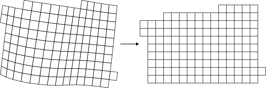
The basic principle of the grid rectification is that a mapping from the distorted image into the rectified image is determined from a distorted image of the rectification grid whose undistorted geometry is well known: The black and white fields of the printed rectification grid are squares (Figure 3).
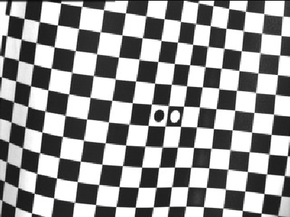 |
In the distorted image, the black and white fields do not appear as squares because of the non-planar object surface, the perspective distortions, and the lens distortions. |
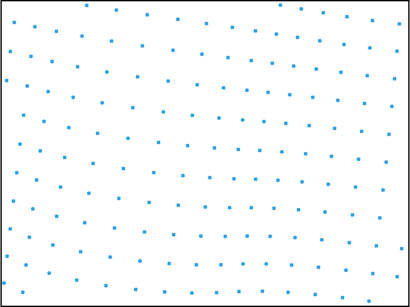 |
First, the corners of the black and white fields must be extracted with the operator saddle_points_sub_pix. |
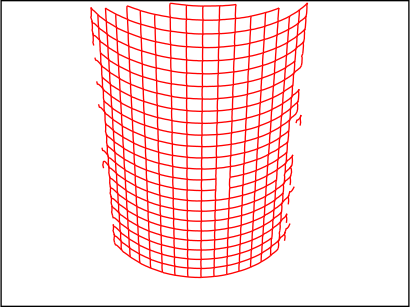 |
These corners must be connected along the borders of the black and white fields with the operator connect_grid_points. |
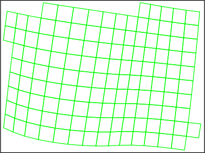 |
Finally, the connecting lines must be combined into meshes with the operator gen_grid_rectification_map, which also determines the mapping for the rectification of the distorted image. |
If you want to use a self-defined grid, the grid points must be defined by yourself.
Then, the operator gen_arbitrary_distortion_map can be used to determine the mapping.
The mapping is determined such that the distorted rectification grid will be mapped into its original undistorted geometry (Figure 4).
With this mapping, any image that shows the same distortions can be rectified easily with the operator map_image.
Note that within the meshes a bilinear interpolation is carried out.
Therefore, it is important to use a rectification grid with an appropriate grid size.
Rules for taking images of the rectification grid🔗
If you want to achieve accurate results, please follow the rules given in this section:
- The image must not be overexposed or underexposed: otherwise, the extraction of the corners of the black and white fields of the rectification grid may fail.
- The contrast between the bright and the dark fields of the rectification grid should be as high as possible.
- Ensure that the rectification grid is homogeneously illuminated.
- The images should contain as little noise as possible.
- The border length of the black and white fields should be at least 10 pixels.
In addition to these few rules for the taking of the images of the rectification grid, it is very important to use a rectification grid with an appropriate grid size because the mapping is determined such that within the meshes of the rectification grid a bilinear interpolation is applied. Because of this, non-linear distortions within the meshes cannot be eliminated.
The use of a rectification grid that is too coarse, i.e., whose grid size is too large, leads to errors in the rectified image (Figure 5).
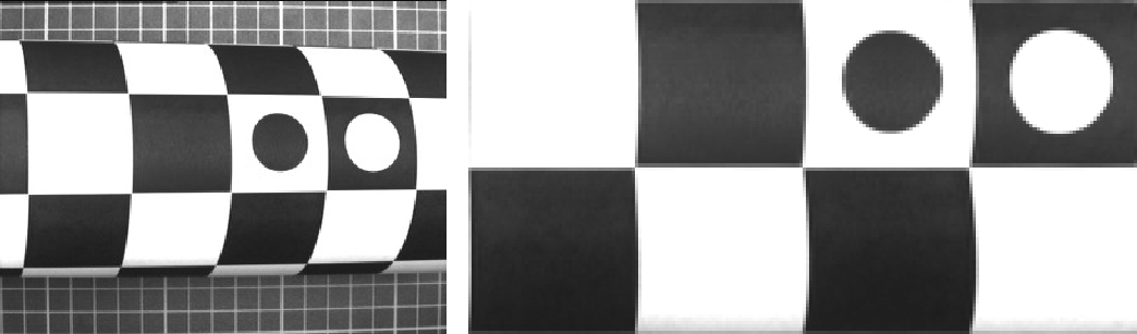
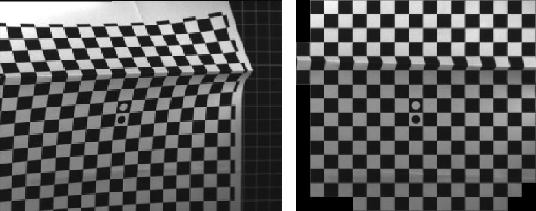
If it is necessary to fold the rectification grid, it should be folded along the borders of the black and white fields. Otherwise, i.e., if the fold crosses these fields, the rectified image will contain distortions because of the bilinear interpolation within the meshes (Figure 6).
Machine vision of ruled surfaces🔗
In this section, the rectification of images of ruled surfaces is described in detail.
Again, the example of the cylindrically shaped object (%HALCONEXAMPLES%\hdevelop\Tools\Grid-Rectification\grid_rectification.hdev) is used to explain the involved operators.
First, the operator create_rectification_grid is used to create a suitable rectification grid.
create_rectification_grid (WidthOfGrid, NumSquares, 'rectification_grid.ps'The parameter WidthOfGrid defines the effectively usable size of the rectification grid in meters and the parameter NumSquares sets the number of squares (black and white fields) per row.
The rectification grid is written to the PostScript file that is specified by the parameter GridFile.
To determine the mapping, an image of the rectification grid, wrapped around the object, must be taken as described here. Figure 7 shows an image of a cylindrical object and the same object wrapped by the rectification grid.
Then, the rectification grid is searched in this image with the operator find_rectification_grid.
find_rectification_grid (Image, GridRegion, MinContrast, Radius)The operator find_rectification_grid extracts image areas with a contrast of at least MinContrast and fills up the holes in these areas.
Note that in this case, contrast is defined as the gray value difference of neighboring pixels in a slightly smoothed copy of the image (Gaussian smoothing with \(\sigma = 1.0\)).
Therefore, the value for the parameter MinContrast must be set significantly lower than the gray value difference between the black and white fields of the rectification grid.
Small areas of high contrast are then eliminated by an opening with the radius Radius.
The resulting region is used to restrict the search space for the following steps with the operator reduce_domain (see Table 2).
reduce_domain (Image, GridRegion, ImageReduced)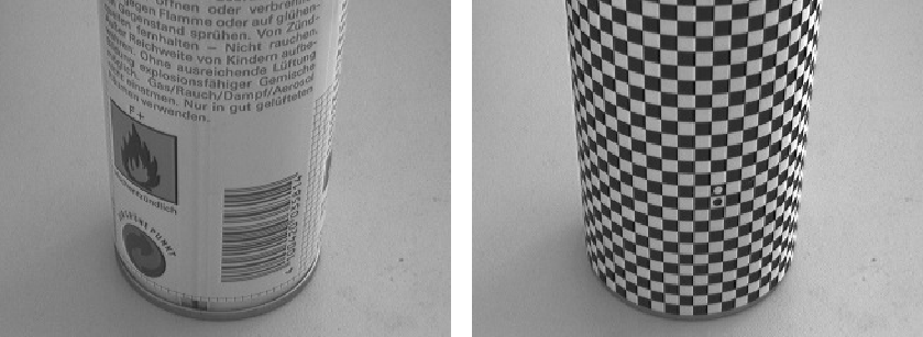
The corners of the black and white fields appear as saddle points in the image.
They can be extracted with the operator saddle_points_sub_pix (see Table 2).
saddle_points_sub_pix (ImageReduced, 'facet', SigmaSaddlePoints, Threshold, Row, Col)The parameter Sigma controls the amount of Gaussian smoothing that is carried out before the actual extraction of the saddle points.
Which point is accepted as a saddle point is based on the value of the parameter Threshold.
If Threshold is set to higher values, fewer but more distinct saddle points are returned than if Threshold is set to lower values.
The filter method that is used for the extraction of the saddle points can be selected by the parameter Filter.
It can be set to 'facet' or 'gauss'.
The method 'facet' is slightly faster.
The method 'gauss' is slightly more accurate but tends to be more sensitive to noise.
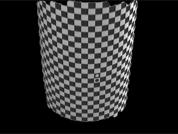 |
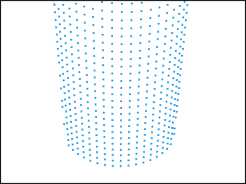 |
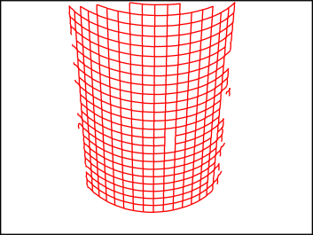 |
|---|---|---|
| Image reduced to the extracted area of the rectification grid | Extracted corners of the black and white fields | Lines that connect the corners |
To generate a representation of the distorted rectification grid, the extracted saddle points must be connected along the borders of the black and white fields (Table 2).
This is done with the operator connect_grid_points.
connect_grid_points (ImageReduced, ConnectingLines, Row, Col, SigmaConnectGridPoints, MaxDist)Again, the parameter Sigma controls the amount of Gaussian smoothing that is carried out before the extraction of the borders of the black and white fields.
When a tuple of three values [sigma_min, sigma_max, sigma_step] is passed instead of only one value, the operator connect_grid_points tests every sigma within the given range from sigma_min to sigma_max with a step size of sigma_step and chooses the sigma that causes the largest number of connecting lines.
The same happens when a tuple of only two values sigma_min and sigma_max is passed.
However, in this case a fixed step size of 0.05 is used.
The parameter MaxDist defines the maximum distance with which an edge may be linked to the respectively closest saddle point.
This helps to overcome the problem that edge detectors typically return inaccurate results in the proximity of edge junctions.
Figure 8 shows the connecting lines if the parameter MaxDist has been selected inappropriately.
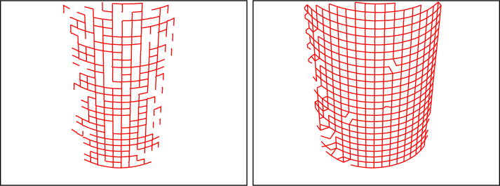
MaxDist selected (Left) too small and (Right) too large. Then, the rectification map is determined from the distorted grid with the operator gen_grid_rectification_map.
gen_grid_rectification_map (ImageReduced, ConnectingLines, Map, Meshes, GridSpacing, 0, Row, Col, 'bilinear')The parameter GridSpacing defines the size of the grid meshes in the rectified image.
Each of the black and white fields is projected onto a square of GridSpacing \(\times\) GridSpacing pixels.
The parameter Rotation controls the orientation of the rectified image.
The rectified image can be rotated by 0, 90, 180, or 270 degrees, or it is rotated such that the black circular mark is left of the white circular mark if Rotation is set to 'auto'.
Using the derived rectification map, any image that shows the same distortions can be rectified very fast with the operator map_image (see Figure 9).
Note that the objects must appears at exactly the same position in the distorted images.
map_image (ImageReduced, Map, ImageMapped)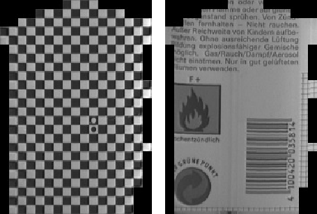
Using self-defined rectification grids🔗
Up to now, we have used the predefined rectification grid together with the appropriate operators for its segmentation. In this section, an alternative to this approach is presented. You can arbitrarily define the rectification grid by yourself, but note that in this case you must also carry out the segmentation by yourself.
This example shows how the grid rectification can be used to generate arbitrary distortion maps based on self-defined grids.
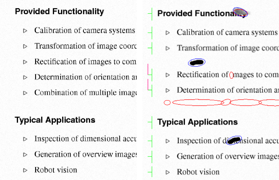
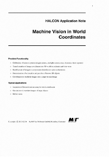
The example application is a print inspection. It is assumed that some parts are missing and that smudges are present. In addition, lines may be vertically shifted, e.g., due to an inaccurate paper transport, i.e., distortions in the vertical direction of the printed document may be present. These distortions should not result in a rejection of the tested document. Therefore, it is not possible to simply compute the difference image between a reference image and the image that must be checked.
Reference and test image
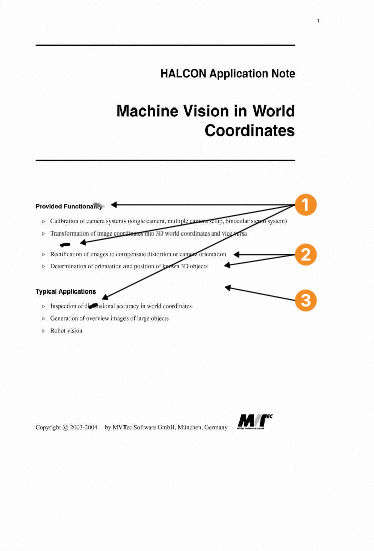
smudges displaced lines missing line
In a first step, the displacements between the lines in the reference document and the test document are determined. With this, the rectification grid is defined. The resulting rectification map is applied to the reference image to transform it into the geometry of the test image. Now, the difference image of the mapped reference image and the test image can be computed.
The example program %HALCONEXAMPLES%\solution_guide\3d_vision\grid_rectification_arbitrary_distortion.hdev uses the shape-based matching to determine corresponding points in the reference image and the test image.
First, the different matching models are generated for every region in the reference image.
Then, the corresponding points are searched in the test image by searching the matches for every model.
Based on the corresponding points of the reference and the test image (RowRef, ColRef, RowTest, and ColTest), the coordinates of the grid points of the distorted grid are determined.
In this example, the row and column coordinates can be determined independently from each other because only the row coordinates are distorted.
Note that the upper left grid point of the undistorted grid is assumed to have the coordinates (-0.5, -0.5).
This means that the corresponding grid point of the distorted grid will be mapped to the point (-0.5, -0.5).
Because there are only vertical distortions in this example, the column coordinates of the distorted grid are equidistant, starting at the value -0.5.
GridSpacing := 10
ColShift := mean(ColTest - ColRef)
RefGridColValues := []
for HelpCol := -0.5 to WidthTest + GridSpacing by GridSpacing
    RefGridColValues := [RefGridColValues,HelpCol + ColShift]
endfor
The row coordinates of the distorted grid are determined by a linear interpolation between the above determined pairs of corresponding row coordinates.
MinValue := 0
MaxValue := HeightTest + GridSpacing
sample_corresponding_values (RowTest, RowRef - 0.5, MinValue, MaxValue, GridSpacing, RefGridRowValues)
The interpolation is performed within the procedure which is part of the example program %HALCONEXAMPLES%\solution_guide\3d_vision\grid_rectification_arbitrary_distortion.hdev.
procedure sample_corresponding_values (Values, CorrespondingValues, MinValue, MaxValue, InterpolationInterval, SampledCorrespondingValues):::Now, the distorted grid is generated row by row.
RefGridRow := []
RefGridCol := []
Ones := gen_tuple_const(|RefGridColValues|,1)
for r := 0 to |RefGridRowValues| - 1 by 1
    RefGridRow := [RefGridRow,RefGridRowValues[r] * Ones]
    RefGridCol := [RefGridCol,RefGridColValues]
endfor
The operator gen_arbitrary_distortion_map uses this distorted grid to derive the rectification map that maps the reference image into the geometry of the test image.
In this case, the reference image is mapped into the geometry of the test image to facilitate the marking of the differences in the test image.
Obviously, the rectification grid can also be defined such that the test image is mapped into the geometry of the reference image.
gen_arbitrary_distortion_map (Map, GridSpacing, RefGridRow, RefGridCol, |RefGridColValues|, WidthRef, HeightRef, 'bilinear')With this rectification map, the reference image can be transformed into the geometry of the test image.
Note that the size of the mapped image depends on the number of grid cells and on the size of one grid cell, which must be defined by the parameter GridSpacing.
Possibly, the size of the mapped reference image must be adapted to the size of the test image.
map_image (ImageRef, Map, ImageMapped)
crop_part (ImageMapped, ImagePart, 0, 0, WidthTest, HeightTest)
Finally, the test image can be subtracted from the mapped reference image.
sub_image (ImagePart, ImageTest, ImageSub, 1, 128)Figure 10 shows the resulting difference image. In this case, missing parts appear dark while the smudges appear bright.
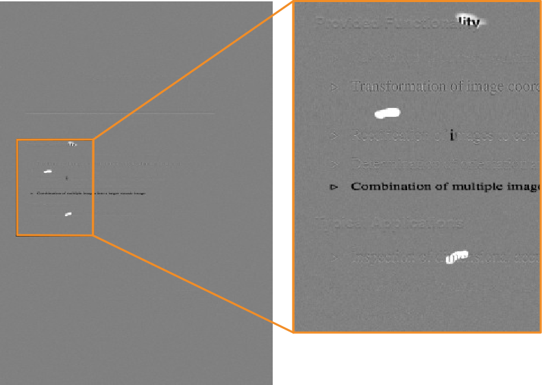
The differences between the test image and the reference image can now be extracted easily from the difference image with the operator threshold.
If the difference image is not needed, e.g., for visualization purposes, the differences can be derived directly from the test image and the reference image with the operator dyn_threshold.
Figure 11 shows the differences in a cut-out of the reference image and of the test image. The calibration marks near the left border indicate the vertical position of the components that were used for the determination of the corresponding points. Vertical shifts of the components with respect to the reference image are indicated by a vertical line of the respective length that is attached to the respective calibration mark. All other differences that could be detected between the test image and the reference image are encircled.