Workflow🔗
Using a single calibration plate🔗
For the first approach, the calibration is performed using a series of images of a single standard HALCON calibration plate with hexagonally arranged marks. Thereby, internal and external camera parameters are determined at once. This approach is quite straightforward, however it only works, if all cameras of a setup can acquire adequate images of the calibration plate simultaneously. Usually this is only the case for a two-camera setup.
The plane, defined by a suitable pose of the calibration plate, that was received during the calibration step, can be used as the rectification plane onto which images from both cameras can then be mapped before they are stitched together.
Calibration🔗
When using a calibration plate with hexagonally arranged marks, the calibration images do not need to contain the entire calibration plate (Figure 1).
Therefore, the following mosaicking approach is suitable, when having a setup where convenient calibration images can be acquired simultaneously by all cameras. Both internal and external camera parameters can be determined within this setup.
After setting initial values for the internal camera parameters with the procedure gen_cam_par_area_scan_division, a calibration data model is created using create_calib_data.
gen_cam_par_area_scan_division (0.012, 0, 4.4e-6, 4.4e-6, WidthCam1 / 2, HeightCam1 / 2, WidthCam1, HeightCam1, StartCamParam1)
gen_cam_par_area_scan_division (0.012, 0, 4.4e-6, 4.4e-6, WidthCam2 / 2, HeightCam2 / 2, WidthCam2, HeightCam2, StartCamParam2)
create_calib_data ('calibration_object', 2, 1, CalibDataID)
set_calib_data_cam_param (CalibDataID, 0, [], StartCamParam1)
set_calib_data_cam_param (CalibDataID, 1, [], StartCamParam2)
set_calib_data_calib_object (CalibDataID, 0, 'calplate_160mm.cpd')
To achieve high accuracy, ten calibration images are taken by each camera. A simultaneous acquisition of the image pairs ensures, that the calibration plate is in the exact same position referring to world coordinates for both calibration images.
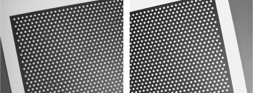
With find_calib_object, the marks of the calibration plate are located and the extracted information is accumulated in the calibration data model for all calibration images.
Using calibrate_cameras the two cameras can be calibrated simultaneously.
for I := 0 to NumCalibImages - 1 by 1
    read_image (ImageCam1, ImagePath + '/calib_cam_1_' + (I + 1)$'02d')
    read_image (ImageCam2, ImagePath + '/calib_cam_2_' + (I + 1)$'02d')
    find_calib_object (ImageCam1, CalibDataID, 0, 0, I, [], [])
    find_calib_object (ImageCam2, CalibDataID, 1, 0, I, [], [])
endfor
calibrate_cameras (CalibDataID, Errors)Mosaicking🔗
After the calibration of the cameras is finished successfully, the setup is now used to acquire images of an object (Figure 2).
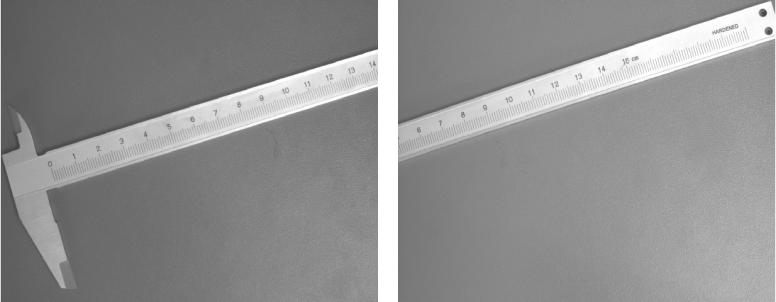
In order to stitch images of the two cameras together, they need to be projected into a rectification plane. Therefore, a reference pose of the calibration plate (while positioned in the same plane as the object) with respect to the first camera is used. In order to take the thickness of the calibration plate into account, the z-component of the pose is adjusted by 4mm. Thus, the rectification plane corresponds to the measurement plane. Then, the relative pose of the second camera with respect to the first camera is inverted and combined with the absolute pose of the first camera in order to get its absolute pose.
get_calib_data (CalibDataID, 'calib_obj_pose', [0, 0], 'pose', Pose1)
set_origin_pose (Pose1, 0, 0, 0.004, Pose1)
get_calib_data (CalibDataID, 'camera', 1, 'pose', RelPose2)
pose_invert (RelPose2, RelPose2Inverted)
pose_compose (RelPose2Inverted, Pose1, Pose2)
Now, after the poses of the rectification plane and the cameras are known, a mapping for the object images is needed.
Therefore, the camera poses have to be adjusted by the particular thickness of the respective object.
Additionally the x- and y-coordinates are adjusted, so the origin of the rectification plane approximately matches the origin of the result image, hence the object will be contained in it entirely.
The mappings are then generated by the operator gen_image_to_world_plane_map.
set_origin_pose (Pose1, -0.14, -0.07, HeightCorrections[OIdx], WorldPose1)
set_origin_pose (Pose2, -0.14, -0.07, HeightCorrections[OIdx], WorldPose2)
gen_image_to_world_plane_map (Map1, CamParam1, WorldPose1, WidthCam1, HeightCam1, TargetWidth, TargetHeight, Scale, 'bilinear')
gen_image_to_world_plane_map (Map2, CamParam2, WorldPose2, WidthCam2, HeightCam2, TargetWidth, TargetHeight, Scale, 'bilinear')
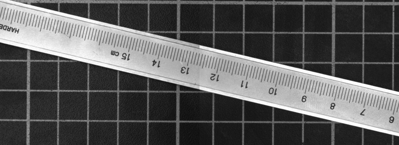
The mappings can be applied with the operator map_image, so both images are projected onto the rectification plane accordingly (see Figure 3).
The mapped images are slightly rotated, as the calibration plate in the image, chosen as reference image in the calibration, was rotated in regard to the image edges as well.
map_image (ImageCam1, Map1, ImageWorld1)
map_image (ImageCam2, Map2, ImageWorld2)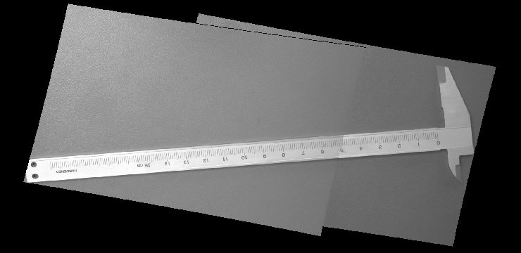
To get a single result image, the mapped images need to be stitched together. When assembling images of a multi-view camera setup, you need to pay attention to overlapping image parts and the image domains.
get_domain (ImageWorld1, Domain1)
get_domain (ImageWorld2, Domain2)
intersection (Domain1, Domain2, RegionIntersection)
paint_region (RegionIntersection, ImageWorld1, ImageWorld1Blackended, 0, 'fill')
full_domain (ImageWorld1Blackended, ImagePart1)
full_domain (ImageWorld2, ImagePart2)
add_image (ImagePart1, ImagePart2, ImageFull, 1, 0)
By adding the two images, gray values of the overlapping parts are added up.
Therefore, in one of the images, the color value of intersecting pixels is set to 0 by using paint_region on the respective image part beforehand.
The domain of both individual images is extended, such that it is identical.
The final step is to remove the black borders.
Therefore, the full image is rotated so that a rectangle, created by the operator gen_rectangle1, can be fitted in to define the new domain of the image with reduce_domain.
This domain is eventually cropped with crop_domain and the image is oriented the favored way by flipping it twice with mirror_image (see final result in Figure 4.
rotate_image (ImageFull, ImageRotated, 12, 'constant')
gen_rectangle1 (RectangleDomain, Borders[0], Borders[1], Borders[2], Borders[3])
reduce_domain (ImageRotated, RectangleDomain, ImageReduced)
crop_domain (ImageReduced, ImageReduced)
mirror_image (ImageReduced, ImageReduced, 'row')
mirror_image (ImageReduced, ImageResult, 'column')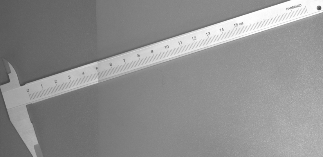
Using multiple calibration plates🔗
The second mosaicking approach is more complex, compared to the first one, but allows you to cover a bigger area, as not all cameras need to have the same calibration plate in their field of view. In fact, in order to perform a measurement task, the images acquired by the cameras do not necessarily have to overlap. Instead of a single calibration plate, a calibration object consisting of multiple calibration plates is used. Thereby, the relative position of the plates to each other must be known very precisely. Internal and external camera parameters are therefore determined separately.
The idea for this approach is to rectify the two images in such a way, that they fit exactly next to each other. This is first done with images showing the calibration plates in order to create the rectification maps for this setup. Those mappings can then be applied to further image pairs.
Calibration🔗
The calibration of the images can be broken down into two separate steps.
The first step is to determine the internal camera parameters for each of the cameras in use. This can be done for each camera independently.
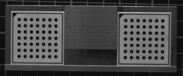
The second step is to determine the external camera parameters for all cameras. Because the final coordinates should refer to one world coordinate system for all images, a big calibration object that appears in all images has to be used. For calibration plates with rectangularly arranged marks, which must be completely visible in the image, we propose to use a calibration object like the one displayed in Figure 5, which consists of as many calibration plates as the number of cameras that are used.
For the determination of the external camera parameters, it is sufficient to use one calibration image from each camera only.
Note that the calibration object must not be moved in between the acquisition of the individual images.
Ideally, the images are acquired simultaneously.
The pose of the calibration plates relative to the cameras is then extracted using an initialized calibration data model and the operators find_calib_object and get_calib_data_observ_points.
CaltabName := 'caltab_30mm.descr'
create_calib_data ('calibration_object', 2, 1, CalibDataID)
set_calib_data_calib_object (CalibDataID, 0, CaltabName)
set_calib_data_cam_param (CalibDataID, 0, [], CamParam1)
set_calib_data_cam_param (CalibDataID, 1, [], CamParam2)
*
* Find and display the calibration plate in the images.
find_calib_object (Image1, CalibDataID, 0, 0, 0, [], [])
get_calib_data_observ_points (CalibDataID, 0, 0, 0, RowCoord1, ColumnCoord1, Index1, Pose1)
*
find_calib_object (Image2, CalibDataID, 1, 0, 0, [], [])
get_calib_data_observ_points (CalibDataID, 1, 0, 0, RowCoord2, ColumnCoord2, Index2, Pose2)
Here, calibration plates with rectangularly arranged marks are used. The calibration is nevertheless easy if standard HALCON calibration plates mounted on some kind of carrier plate are used such that in each image one calibration plate is completely visible. An example for such a calibration object for a two-camera setup is given in Figure 5. The respective calibration images for the determination of the external camera parameters are shown in Figure 6. Note that the relative position of the calibration plates with respect to each other must be known precisely. This can be done with different approaches described here.
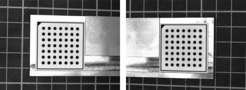
Note also that only the relative position of the calibration marks among each other shows high accuracy but not the borders of the calibration plate. The rows of calibration marks may be slanted with respect to the border of the calibration plate and even the distance of the calibration marks from the border of the calibration plate may vary. Therefore, aligning the calibration plates along their boundaries may result in a shift in x- and y-direction with respect to the coordinate system of the calibration plate in its initial position.
Merging the individual images into one larger image🔗
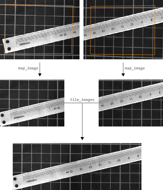
At first, the individual images must be rectified, i.e., transformed so that they exactly fit together.
This can be achieved by using the operators gen_image_to_world_plane_map and map_image.
Then, the mosaic image can be generated by the operator tile_images, which tiles multiple images into one larger image.
These steps are visualized in Figure 7.
In the following, we will only discuss the problem of defining the appropriate image detail, i.e., the position of the upper left corner and the size of the rectified images. Again, the description is based on the two-camera setup.
Defining the rectification of the first image🔗
For the first (here: left) image, the determination of the necessary shift of the pose is straightforward. You can define the upper left corner of the rectified image in image coordinates, e.g., interactively or, as in the example program, based on a preselected border width.
UpperRow := HeightImage1 * BorderInPercent / 100.0
LeftColumn := WidthImage1 * BorderInPercent / 100.0
Then, this point must be transformed into world coordinates.
image_points_to_world_plane (CamParam1, Pose1, UpperRow, LeftColumn, 'm', LeftX, UpperY)The resulting coordinates can be used directly, together with the shift that compensates the thickness of the calibration plate to modify the origin of the world coordinate system in the left image.
set_origin_pose (Pose1, LeftX, UpperY, DiffHeight, PoseNewOrigin1)This means that we shift the origin of the world coordinate system from the origin of the calibration plate to the position that defines the upper left corner of the rectified image (Figure 8).
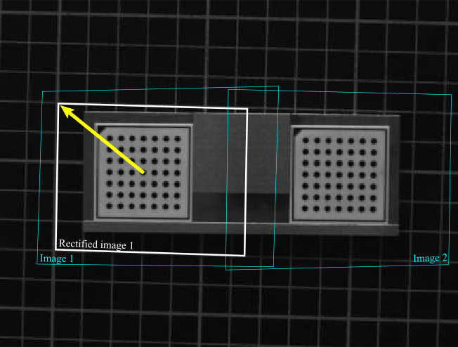
White: rectified images
Turquoise: original images
The size of the rectified image, i.e., its width and height, can be determined from points originally defined in image coordinates, too. In addition, the desired pixel size of the rectified image must be specified.
PixelSize := 0.0001For the determination of the height of the rectified image we need to define a point that lies near the lower border of the first image.
LowerRow := HeightImage1 * (100 - BorderInPercent) / 100.0Again, this point must be transformed into the world coordinate system.
image_points_to_world_plane (CamParam1, Pose1, LowerRow, LeftColumn, 'm', X1, LowerY)The height can be determined as the vertical distance between the upper left point and the point near the lower image border, expressed in pixels of the rectified image.
HeightRect := int((LowerY - UpperY) / PixelSize)Analogously, the width can be determined from a point that lies in the overlapping area of the two images, i.e., near the right border of the first image.
RightColumn := WidthImage1 * (100 - OverlapInPercent / 2.0) / 100.0
image_points_to_world_plane (CamParam1, Pose1, UpperRow, RightColumn, 'm', RightX, Y1)
WidthRect := int((RightX - LeftX) / PixelSize)
Note
The above described definitions of the image points, from which the upper left corner and the size of the rectified image are derived, assume that the x- and y-axes of the world coordinate system are approximately aligned to the column- and row-axes of the first image. This can be achieved by placing the calibration plate in the first image approximately aligned with the image borders. Otherwise, the distances between the above mentioned points make no sense and the upper left corner and the size of the rectified image must be determined in a manner that is adapted for the configuration at hand.
With the shifted pose and the size of the rectified image, the rectification map for the first image can be derived.
gen_image_to_world_plane_map (MapSingle1, CamParam1, PoseNewOrigin1, Width, Height, WidthRect, HeightRect, PixelSize, 'bilinear')Defining the rectification of the second image🔗
The second image must be rectified such that it fits exactly to the right of the first rectified image. This means that the upper left corner of the second rectified image must be identical with the upper right corner of the first rectified image. Therefore, we need to know the coordinates of the upper right corner of the first rectified image in the coordinate system that is defined by the calibration plate in the second image.
First, we express the upper right corner of the first rectified image in the world coordinate system that is defined by the calibration plate in the first image. It can be determined by a transformation from the origin into the upper left corner of the first rectified image (a translation in the example program) followed by a translation along the upper border of the first rectified image. Together with the shift that compensates the thickness of the calibration plate, this transformation is represented by the homogeneous transformation matrix \(\mvHomMatrixVar{cp1}{ur1}\) (see Figure 9), which can be defined by:
hom_mat3d_translate_local (HomMat3DIdentity, LeftX + PixelSize * WidthRect, UpperY, DiffHeight, cp1Hur1)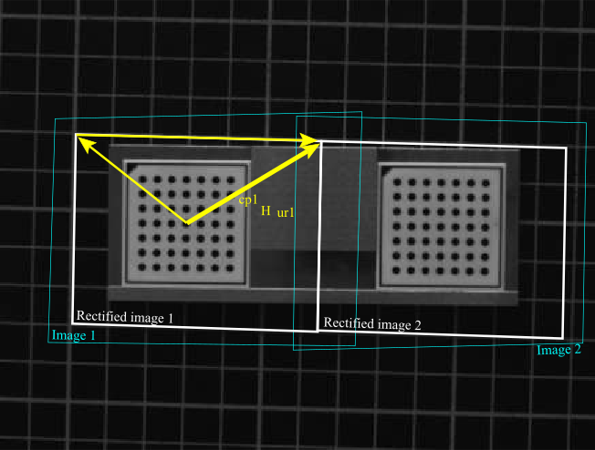
White: rectified images
Turquoise: original images
Then, we need the transformation between the two calibration plates of the calibration object. The homogeneous transformation matrix \(\mvHomMatrixVar{cp1}{cp2}\) describes how the world coordinate system defined by the calibration plate in the first image is transformed into the world coordinate system defined by the calibration plate in the second image (Figure 10). This transformation must be known beforehand from a precise measurement of the calibration object.
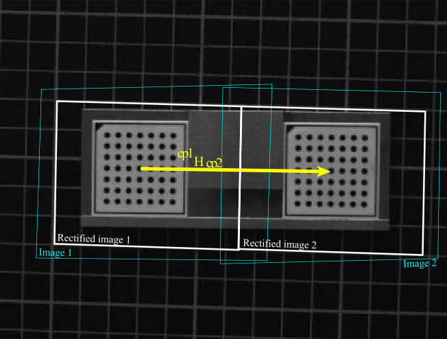
White: rectified images
Turquoise: original images
From these two transformations, it is easy to derive the transformation that transforms the world coordinate system of the second image such that its origin lies in the upper left corner of the second rectified image. For this, the two transformations have to be combined appropriately (see Figure 11):
This can be implemented as follows:
hom_mat3d_invert (cp1Hcp2, cp2Hcp1)
hom_mat3d_compose (cp2Hcp1, cp1Hur1, cp2Hul2)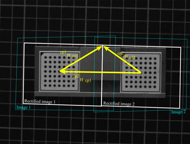
White: rectified images
Turquoise: original images
With this, the pose of the calibration plate in the second image can be modified such that the origin of the world coordinate system lies in the upper left corner of the second rectified image.
pose_to_hom_mat3d (Pose2, cam2Hcp2)
hom_mat3d_compose (cam2Hcp2, cp2Hul2, cam2Hul2)
hom_mat3d_to_pose (cam2Hul2, PoseNewOrigin2)
With the resulting new pose and the size of the rectified image, which can be the same as for the first rectified image, the rectification map for the second image can be derived.
gen_image_to_world_plane_map (MapSingle2, CamParam2, PoseNewOrigin2, Width, Height, WidthRect, HeightRect, PixelSize, 'bilinear')Rectifying the images🔗
Once the rectification maps are created, every image pair from the two-camera setup can be rectified and tiled very efficiently. The resulting mosaic image consists of the two rectified images and covers a part as indicated in Figure 12}.

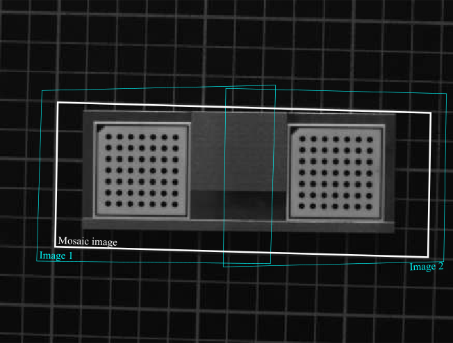
White: mosaic image
Turquoise: original images
///
The rectification is carried out by the operator map_image.
map_image (Image1, MapSingle1, RectifiedImage1)
map_image (Image2, MapSingle2, RectifiedImage2)
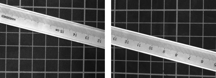
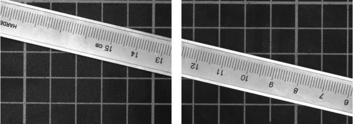
This transforms the two images displayed in Figure 13, into the two rectified images that are shown in Figure 14.
Test images and rectified images
As a preparation for the tiling, the rectified images must be concatenated into one tuple, which then contains both images.
concat_obj (RectifiedImage1, RectifiedImage2, Concat)Then the two images can be tiled.
tile_images (Concat, Combined, 2, 'vertical')The resulting mosaic image is displayed in Figure 15.