3D transformation matrixes and homogenous transformation matrices🔗
Transformations using 3D transformation matrices🔗
Translation🔗
Translation of points
In Figure 1, our example point has been translated along the x-axis of the camera coordinate system.
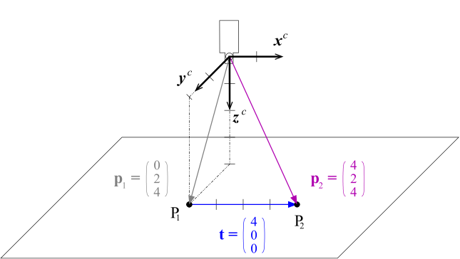
Camera coordinate system: \((x^c, y^c, z^c)\)
The coordinates of the resulting point \(P_2\) can be calculated by adding two vectors, the coordinate vector \(p_1\) of the point and the translation vector \(t\):
Multiple translations are described by adding the translation vectors. This operation is commutative, i.e., the sequence of the translations has no influence on the result.
Translation of coordinate systems
Coordinate systems can be translated just like points. In the example in Figure 2, the coordinate system \(c_1\) is translated to form a second coordinate system, \(c_2\). Then, the position of \(c_2\) in \(c_1\), that is, the coordinate vector of its origin relative to \(c_1\) (\(o^{c1}_{c2}\)), is identical to the translation vector:
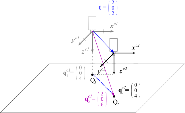
Camera coordinate system 1: \((x^{c1}, y^{c1}, z^{c1})\)
Camera coordinate system 2: \((x^{c2}, y^{c2}, z^{c2})\)
Coordinate transformations
In fact, the translation of a point can also be thought of as translating it together with its local coordinate system. This is depicted in Figure 2: The coordinate system \(c_1\), together with the point \(Q_1\), is translated by the vector \(t\), resulting in the coordinate system \(c_2\) and the point \(Q_2\). The points \(Q_1\) and \(Q_2\) then have the same coordinates relative to their local coordinate system, i.e., \(q^{c1}_{1} = q^{c2}_{2}\).
If coordinate systems are only translated relative to each other, coordinates can be transformed very easily between them by adding the translation vector:
Figure 2 visualizes this equation: \(q^{c1}_2\), that is, the coordinate vector of \(Q_2\) in the coordinate system \(c_1\), is composed by adding the translation vector \(t\) and the coordinate vector of \(Q_2\) in the coordinate system \(c_2\) (\(q^{c2}_2\)).
The downside of this graphical notation is that, at first glance, the direction of the translation vector appears to be contrary to the direction of the coordinate transformation: The vector points from the coordinate system \(c_1\) to \(c_2\), but transforms coordinates from the coordinate system \(c_2\) to \(c_1\). According to this, the coordinates of \(Q_1\) in the coordinate system \(c_2\), that is, the inverse transformation, can be obtained by subtracting the translation vector from the coordinates of \(Q1\) in the coordinate system \(c_1\):
Summary
-
Points are translated by adding the translation vector to their coordinate vector. Analogously, coordinate systems are translated by adding the translation vector to the position (coordinate vector) of their origin.
-
To transform point coordinates from a translated coordinate system \(c_2\) into the original coordinate system \(c_1\), you apply the same transformation to the points that was applied to the coordinate system, that is, you add the translation vector used to translate the coordinate system \(c_1\) into \(c_2\).
-
Multiple translations are described by adding all translation vectors; the sequence of the translations does not affect the result.
Rotation🔗
Rotation of points
In Figure 3, the point \(p_1\) is rotated by \(-90°\) around the z-axis of the camera coordinate system.
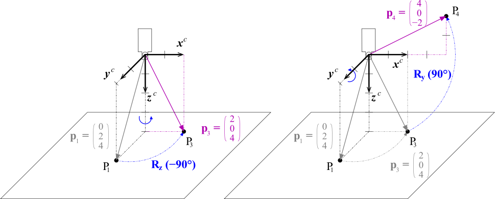
Rotating a point is expressed by multiplying its coordinate vector with a 3 × 3 rotation matrix \(R\). A rotation around the z-axis looks as follows:
Rotations around the x- and y-axis correspond to the following rotation matrices:
Chains of rotations
In Figure 4 the rotated point is further rotated around the y-axis. Such a chain of rotations can be expressed very elegantly by a chain of rotation matrices
Note that in contrast to a multiplication of scalars, the multiplication of matrices is not commutative, i.e., if you change the sequence of the rotation matrices, you get a different result.
Rotation of coordinate systems
In contrast to points, coordinate systems have an orientation relative to other coordinates systems. This orientation changes when the coordinate system is rotated. For example, in Figure 4 the coordinate system \(c_3\) has been rotated around the y-axis of the coordinate system \(c_1\), resulting in a different orientation of the camera. Note that in order to rotate a coordinate system in your mind’s eye, it may help to image the points of the axis vectors being rotated.
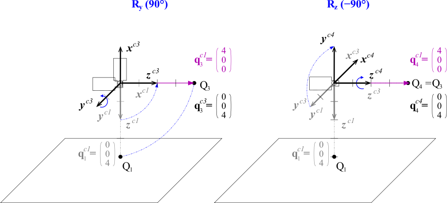
Camera coordinate system 1: \((x^{c1}, y^{c1}, z^{c1})\)
Camera coordinate system 3: \((x^{c3}, y^{c3}, z^{c3})\)
Camera coordinate system 4: \((x^{c4}, y^{c4}, z^{c4})\)
Just like the position of a coordinate system can be expressed directly by the translation vector, the orientation is contained in the rotation matrix: The columns of the rotation matrix correspond to the axis vectors of the rotated coordinate system in coordinates of the original one:
For example, the axis vectors of the coordinate system \(c_3\) in Figure 4 can be determined from the corresponding rotation matrix \(R_y(90°)\) as shown in the following equation; you can easily check the result in the figure.
Coordinate transformation
Like in the case of translation, to transform point coordinates from a rotated coordinate system \(c_3\) into the original coordinate system \(c_1\), you apply the same transformation to the points that was applied to the coordinate system \(c_3\), that is, you multiply the point coordinates with the rotation matrix used to rotate the coordinate system \(c_1\) into \(c_3\):
This is depicted in Figure 4 also for a chain of rotations, which corresponds to the following equation:
In which sequence and around which axes are rotations performed?
If you compare the chains of rotations in Figure 3 and Figure 4 and the corresponding equations, you will note that two different sequences of rotations are described by the same chain of rotation matrices: In Figure 3, the point was rotated first around the z-axis and then around the y-axis, whereas in Figure 4 the coordinate system is rotated first around the y-axis and then around the z-axis. Yet, both are described by the chain \(R_y(\beta) \cdot R_z(\gamma)\)!
The solution to this seemingly paradox situation is that in the two examples the chain of rotation matrices can be “read” in different directions: In Figure 3 it is read from the right to left, and in Figure 4 from left to the right.
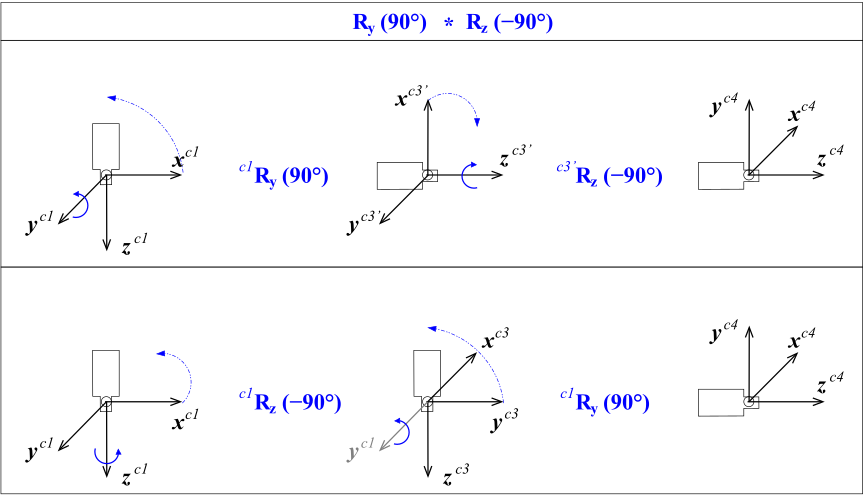
However, there still must be a difference between the two sequences because, as we already mentioned, the multiplication of rotation matrices is not commutative. This difference lies in the second question in the title, that is, around which axes the rotations are performed.
Let’s start with the second rotation of the coordinate system in Figure 4. Here, there are two possible sets of axes to rotate around: those of the “old” coordinate system \(c_1\) and those of the already rotated, “new” coordinate system \(c_3\). In the example, the second rotation is performed around the “new” z-axis.
In contrast, when rotating points as in Figure 3, there is only one set of axes around which to rotate: those of the “old” coordinate system.
From this, we derive the following rules:
-
When reading a chain from the left to right, rotations are performed around the “new” axes.
-
When reading a chain from the right to left, rotations are performed around the “old” axes.
As already remarked, point rotation chains are always read from right to left. In the case of coordinate systems, you have the choice how to read a rotation chain. In most cases, however, it is more intuitive to read them from left to right.
Figure 5 shows that the two reading directions really yield the same result.
Rigid transformations using homogeneous transformation matrices🔗
Rigid transformation of points
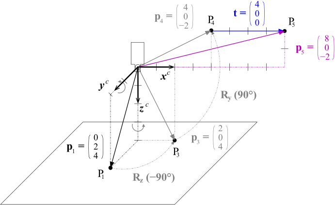
If you combine translation and rotation, you get a so-called rigid transformation. For example, in Figure 6, the translation and rotation of the point from Figure 1 and Figure 3 are combined. Such a transformation is described as follows:
For multiple transformations, such equations quickly become confusing, as the following example with two transformations shows:
An elegant alternative is to use so-called homogeneous transformation matrices and the corresponding homogeneous vectors. A homogeneous transformation matrix $$ contains both the rotation matrix and the translation vector. For example, the rigid transformation can be rewritten as follows:
The usefulness of this notation becomes apparent when dealing with sequences of rigid transformations, which can be expressed as chains of homogeneous transformation matrices, similarly to the rotation chains:
As explained for chains of rotations, chains of rigid transformation can be read in two directions. When reading from left to right, the transformations are performed around the “new” axes, when read from right to left around the “old” axes.
In fact, a rigid transformation is already a chain, since it consists of a translation and a rotation:
If the rotation is composed of multiple rotations around axes as in Figure 6, the individual rotations can also be written as homogeneous transformation matrices:
Reading this chain from right to left, you can follow the transformation of the point in Figure 6: First, it is rotated around the z-axis, then around the (``old’‘) y-axis, and finally it is translated.
Rigid transformation of coordinate systems
Rigid transformations of coordinate systems work along the same lines as described for a separate translation and rotation. This means that the homogeneous transformation matrix \(\mvHomMatrixVar{c1}{c5}\) describes the transformation of the coordinate system \(c_1\) into the coordinate system \(c_5\). At the same time, it describes the position and orientation of coordinate system \(c_5\) relative to coordinate system \(c_1\): Its column vectors contain the coordinates of the axis vectors and the origin.
As already noted for rotations, chains of rigid transformations of coordinate systems are typically read from left to right. Thus, the chain above can be read as first translating the coordinate system, then rotating it around its “new” y-axis, and finally rotating it around its “newest” z-axis.
Coordinate transformations
As described for the separate translation and the rotation, to transform point coordinates from a rigidly transformed coordinate system \(c_5\) into the original coordinate system \(c_1\), you apply the same transformation to the points that was applied to the coordinate system \(c_5\), that is, you multiply the point coordinates with the homogeneous transformation matrix:
Typically, you leave out the homogeneous vectors if there is no danger of confusion and simply write:
Summary
-
Rigid transformations consist of a rotation and a translation. They are described very elegantly by homogeneous transformation matrices, which contain both the rotation matrix and the translation vector.
-
Points are transformed by multiplying their coordinate vector with the homogeneous transformation matrix.
-
If you transform a coordinate system, the homogeneous transformation matrix describes the coordinate system’s resulting position and orientation: The column vectors of the matrix correspond to the axis vectors and the origin of the coordinate system in coordinates of the original one. Thus, you could say that a homogeneous transformation matrix “is” the position and orientation of a coordinate system.
-
To transform point coordinates from a rigidly transformed coordinate system \(c_5\) into the original coordinate system \(c_1\), you apply the same transformation to the points that was applied to the coordinate system, that is, you multiply them with the homogeneous transformation matrix that was used to transform the coordinate system \(c_1\) into \(c_5\).
-
Multiple rigid transformations are described by a chain of transformation matrices, which can be read in two directions. When read from left to the right, rotations are performed around the “new” axes; when read from the right to left, the transformations are performed around the “old” axes.
HALCON operators
Homogeneous transformation matrices are the answer to all our questions regarding the use of 3D coordinates. Because of this, they form the basis for HALCON’s operators for 3D transformations. Below, you find a brief overview of the relevant operators.
-
hom_mat3d_identitycreates the identity transformation. -
hom_mat3d_translatetranslates along the “old” axes: \(H_2 = H(t) \cdot H_1\) -
hom_mat3d_translate_localtranslates along the “new” axes: \(H_2 = H_1 \cdot H(t)\) -
hom_mat3d_rotaterotates around the “old” axes: \(H_2 = H(R) \cdot H_1\) -
hom_mat3d_rotate_localrotates around the “new” axes: \(H_2 = H_1 \cdot H(R)\) -
hom_mat3d_composemultiplies two transformation matrices: \(H_3 = H_1 \cdot H_2\) -
hom_mat3d_invertinverts a transformation matrix: \(H_2 = H_1^{-1}\) -
affine_trans_point_3dtransforms a point using a transformation matrix: \(p_2 = H_0 \cdot p_1\)